WeвҖҷve been on a raster data format journey lately on our blog. Most recently we did a compression deep dive, and we spent two posts before that digging into the tyranny of chunking and the history of chunked raster formats. If we go all the way back to our first post вҖңIs Zarr the new COG?вҖқ, however, itвҖҷs interesting to remember that we started this whole thing off with a profound pronouncement: вҖңNo. Despite what you may have heard, Zarr is not (yet) a replacement for the Cloud-Optimized GeoTIFF (COG) format.”
While we may have unintentionally ruffled some feathers with that statement, we still stand by it. Why? Well, we have several reasons, but perhaps the biggest is because of metadata!
WeвҖҷll start by getting a bit philosophical about what, exactly, constitutes metadata. Once we develop an effective working definition for metadata, weвҖҷll look at how COG and Zarr each represent it. Then, weвҖҷll take a deeper look at various ways geospatial coordinate metadata can be represented across different formats. Next weвҖҷll cover where metadata should be stored: in the file with the data, externally, or both? Finally weвҖҷll talk about data formats, tooling, and conclude with a discussion regarding the utmost importance of conventions for declaring and determining compatibility and enabling interoperability.
What even is metadata?
This is an excellent question, and the answer is not as straightforward as it might seem. A simple response could be something like, вҖңmetadata is information that helps you understand how to interpret data.вҖқ And while that is not a wrong answer, per se, it is also not particularly nuanced.
The line between data and metadata is a particularly fuzzy one. To riff on a famous cliche: вҖңone personвҖҷs metadata is another personвҖҷs data.вҖқ Now, in some cases, especially when considering geospatial raster data, we have a clear delineation: data in COG, metadata in STAC, for example.
Now letвҖҷs say you take a stack of COGs and build them into a datacube, then store that in Zarr. What happens to the metadata? We had a STAC Item per COG before, now we might have a STAC Collection for our ZarrвҖ”or is it an Item? Either way, weвҖҷve lost resolution in our metadata. We end up having to aggregate our metadata values to reflect the total contents of the Zarr, instead of the individual COGs that went into it. In some cases this aggregation is lossless: if every COG had the same value for a metadata fieldвҖ“maybe producer, sensor, or platformвҖ“then aggregating that field to the datacube doesnвҖҷt lose any fidelity.
But other metadata fields, ones with heterogeneous values, are lossily aggregated. Take an example like start and end datetime. Perhaps each COG has its own start and end datetime; with what start and end datetime, then, does our datacube end up? Is it the start datetime of the first COG and the end datetime of the last? WeвҖҷve lost fidelity.
LetвҖҷs imagine going the other way. Pretend we have infinite storage and infinite compute, how might we store metadata? For a raster dataset, we could project our metadata values down to each and every cell, making them additional data variables in the array. Before saying thatвҖҷs crazy and weвҖҷd never do that because it has no value, letвҖҷs take a look at the start and end datetime example again.
Think about a simple example: a whisk broom sensor (for those unfamiliar with the concept, NASA has two fantastic animations that show the difference in how pushbroom vs whisk broom sensors capture data). If we have a scene from said sensor, we normally think of the start and end datetimes as when the first scanline started and the last scanline finished, respectively. But really, when we break it down and consider how the scene was physically captured, we see that each and every cell in the scene has a different start and end datetime! Even at the individual scene level, we see fidelity loss due to the aggregation of these values into metadata. So if we wanted to be really accurate, we could add another dimension to our array with an interval type, and store the start and end times per cell in it.
When viewing metadata this way, as simply additional variables in a dataset, we start to see the fuzziness, the ambiguity, in that line between metadata and data. Metadata and data are not inherently separate. We end up having to separate them though, because we do not have infinite compute and infinite storage. The example aggregations above are a form of compression, which we see can be lossless or lossy depending on the values involved. Compressing the metadata in this way makes it much more compact, and means we end up using a tabular or object format to model the metadata instead of an array. Both transformations make the metadata more efficient for computation and storage.
Just as we see multiscale representation of raster dataвҖ“such as reduced-resolution overviews or pyramidsвҖ“we can also see the potential for multiscale metadata. In fact, we see this concept in STAC already, where Collection-level metadata is intended and expected to be an aggregation of the metadata belonging to each individual Item it contains. And, as our whisk broom illustration shows, Item-level metadata is the roll up of all the metadata for cells in the ItemвҖҷs array. Following this pattern, we end up with a tree, which is a particularly useful and efficient structure for search, to enable us to ultimately arrive at the set of cells we need for our use case.
It is perhaps too bad though that raster data formats have not realized the potential benefits of supporting hierarchical metadata. The reason why is not clear, but it could be something that might be termed вҖңprecedent blindnessвҖқ: historically, querying raster data from a file has been done via coordinate dimensions alone. ThatвҖҷs the whole point of CNG formats like COG and Zarr; users say, вҖңI want data within this coordinate regionвҖқ, and they only have to read tiles that fall within those coordinate bounds. But, raster data usage is not limited to just coordinate-based access patterns. ItвҖҷs easy to imagine a scenario where we might want to query on the data values themselves. Maybe we have a global temperature dataset and we want to see all cells with a temperature greater than 30В° C. We have no means of filtering the chunks we have to read, because spatially we have not restricted our query, so we have to read the whole dataset, every chunk. If we had chunk-level statistics, however, weвҖҷd be able to skip any chunks with a max value less than 30В° C.
Raster data and tabular data are really not any different, at least at a conceptual level. They both define a hypercubic value space. Raster data just tends to be dense within this space, and tabular data tends towards sparseness. For computational and storage efficiency we end up modeling them in these different ways. But, if we recognize these similarities, it is interesting to see that a tabular format like Parquet offers a clear example of hierarchical metadata, allowing for metadata at multiple levels within a table: at the partition (file) level, row group level, column chunk level, and ultimately the data page (analogous to a chunk in a raster format) level. And, with sparse tabular values, the metadata is truly needed at all these levels to facilitate efficient data access by allowing readers to skip chunks that do not have values they want via predicate pushdown.
In the typically-dense space of rasters, the precedent of coordinate-based filtering via chunk coordinates has led us into complacency. Adding additional metadata levels could allow for much more efficient data access patterns. With the increasing need to access data over a network, bringing additional dimensions of predicate pushdown to raster data access could bring significant efficiency improvements to many real access patterns. After all, analytics workflows typically donвҖҷt just want to get all data in an area, they want to do something with that data based on the data values, and not all values may be needed. But, tools don’t expose chunk-level data access filtering because formats don’t support it, and users don’t know to ask for it.
Meanwhile, back on the groundвҖҰ
But still, conceptually, where does data end and metadata begin? Is there really even any distinction?
Matt Hanson, when talking about STAC, likes to point out that STAC has two types of metadata: that for search and discovery to help users find what they are looking for, and that for usability to help tooling better use the data pointed to by a STAC record. The former category of metadata is like the platform or sensor or start and end datetimes; values like we discussed above that are hard to distinguish from data once you look at them for long enough. But, the latter category, the metadata that tells you how to use the data, which gets back to our idea that вҖңmetadata is information that helps you understand how to interpret data.вҖқ
Throughout this series weвҖҷve talked about a number of raster data formats, namely TIFF and Zarr, but also HDF5, NetCDF, and FITS. These are all self-describing raster formats. So far in our posts weвҖҷve primarily been focusing on the вҖңrasterвҖқ part of вҖңraster format,вҖқ but for the rest of this post weвҖҷre going to dig into that вҖңself-describingвҖқ part. By self-describing we mean these formats include information that tells us how to unpack and understand the binary data they contain. While we’ve just shown that metadata is a complex and nuanced topic that deserves more consideration than it may often get, from here on out when we talk about metadata we mean specifically the information in these formats that tells us how to use the data they contain.
Examining file metadata through TIFF and Zarr
So then, what goes into this file metadata? For an example, letвҖҷs look at the Sentinel-2 red band array from way back in our вҖңIs Zarr the new COG?вҖқ post.
TIFF metadata
Here is the metadata stored in our Sentinel-2 COG (specifically the portion for IFD0, the full-resolution array, and not the overviews):
0001030001000000e42a0000
0101030001000000e42a0000
020103000100000010000000
030103000100000008000000
060103000100000001000000
150103000100000001000000
1c0103000100000001000000
3d0103000100000002000000
420103000100000000040000
430103000100000000040000
440104007900000058070000
45010400790000003c090000
530103000100000001000000
0e830c0003000000ca030000
82840c0006000000e2030000
af8703002000000012040000
b18702001e00000052040000
80a4020020020000aa010000
81a402000200000030000000
Admittedly, the above is unlikely to be helpful for most of us. TIFF uses a binary format to store tags and their values, very much in a key/value style, so we represent each of the 19 binary-format tags that are set for this IFD here in hexadecimal. The technical details donвҖҷt much matter for the sake of this discussion (but if you want to dig deeper, including into the process outlined below for reading a tile, check out this notebook), so letвҖҷs skip them and jump directly to a more useful representation of this metadata:
ImageWidth: 10980
ImageLength: 10980
BitsPerSample: 16
Compression: 8
PhotometricInterpretation: 1
SamplesPerPixel: 1
PlanarConfiguration: 1
Predictor: 2
TileWidth: 1024
TileLength: 1024
TileOffsets: (55962680, 57411167, 58810332, 60222446, 616510...
TileByteCounts: (1448479, 1399157, 1412106, 1428549, 1403985...
SampleFormat: 1
ModelPixelScaleTag: (10.0, 10.0, 0.0)
ModelTiepointTag: (0.0, 0.0, 0.0, 600000.0, 5100000.0, 0.0)
GeoKeyDirectoryTag: (1, 1, 0, 7, 1024, 0, 1, 1, 1025, 0, 1, ...
GeoAsciiParamsTag: WGS 84 / UTM zone 10N|WGS 84|
GDAL_METADATA:
  <GDALMetadata>
    <Item name="OVR_RESAMPLING_ALG">AVERAGE</Item>
    <Item name="STATISTICS_MAXIMUM" sample="0">17408</Item>
    <Item name="STATISTICS_MEAN" sample="0">1505.1947339533<...
    <Item name="STATISTICS_MINIMUM" sample="0">294</Item>
    <Item name="STATISTICS_STDDEV" sample="0">659.2450361643...
    <Item name="STATISTICS_VALID_PERCENT" sample="0">99.999<...
    <Item name="OFFSET" sample="0" role="offset">-0.10000000...
    <Item name="SCALE" sample="0" role="scale">0.00010000000...
  </GDALMetadata>
GDAL_NODATA: 0
Now that we can actually see whatвҖҷs going on here, letвҖҷs group these tags into categories:
- where to find particular bits of data on disk:
ImageWidth, ImageLength, TileWidth, TileLength, TileOffsets, TileByteCounts - how to decode the data into numbers:
Compression, PhotometricInterpretation, Predictor, SampleFormat, BitsPerSample, SamplesPerPixel, PlanarConfiguration, GDAL_METADATA.OFFSET, GDAL_METADATA.SCALE, GDAL_NODATA - where the data is in 2D space:
ModelPixelScaleTag, ModelTiepointTag - where the data is on the earth:
GeoKeyDirectoryTag, GeoAsciiParamsTag - statistics summarizing the array:
GDAL_METADATA.STATISTICS_*
Notably, almost all of these tags are necessary for using the data at all. Broadly they tell us where to find the bits of data on disk, what those bits mean, and where they are on the globe. The tags that describe how to find what bytes we want and get data values out of those bytes are part of the core TIFF specification. The coordinate information is part of the GeoTIFF specification that layers on top of TIFF, and the GDAL-related tags are convention, not specification, used by GDAL and compatible tooling. That this is a COG and not just a regular GeoTIFF is not expressed here in just this IFD0 metadata, but is more a matter of file structure.
We can use the geo-related metadata to identify what parts of this imageвҖ“which tilesвҖ“we want to read. LetвҖҷs set that idea aside for the moment though, and focus on how we can use the TIFF-related tags to read tiles out of the file once weвҖҷve identified which one(s) we want.
That is, for a given tile coordinate (x, y) in the tile grid, to read its bytes from the file we first need to convert that two-dimensional coordinate into the linear index of the tile in the file. To do so we need to use the TileWidth and TileLength with our ImageWidth and ImageLength to determine the tileвҖҷs position in row-major order. Then we look up the values in TileOffsets and TileByteCounts at that index to get the byte offset and length of the tile, respectively. With those, we can read said bytes, giving us the compressed bytes for the tile. Now we need to decompress them.
The decompression process requires two of the tags: Compression and Predictor. The former gives us the entropy codec used as the final compression step in the compression process, and the predictor tells us what, if any, processing step was done prior to compression to increase the compressibility of the data (for an in-depth look at these topics see our previous post on compression). Knowing what was done during compression means we can reverse those transformations, giving us the uncompressed bytes of the tile.
WeвҖҷre still not done. We need even more information to be able to make any sense of those bytes. The first thing we need here is BitsPerSample. This tells us how many bits in the bytes correspond to each value. SampleFormat tells us the type of each value (signed integer, unsigned integer, float, complex, etc.). Also we might have more than one value per cell, which is indicated to us by the tags: SamplesPerPixel, PlanarConfiguration, and PhotometricInterpretation.
Notice how much of this process is based on a priori knowledge of enums and procedures from the TIFF specification and is not described in the metadata itself. So, while the metadata is self-describing, it is only so to a point. We lack flexibility, but that is to maintain compatibility with existing tooling, tooling that knows how to interpret these particular tags. That is, we can only use compressors that are part of the Compression enum, and we canвҖҷt have chunks with more than two-dimensions because the spec lacks tags to indicate dimensions beyond length and width. We could use custom tags or values to encode these things, or use other fields in atypical waysвҖ“TIFF alone is quite flexible in this regardвҖ“but then we will have diverged from convention and existing tooling will not be able to read our TIFF. Would it then even be a TIFF? ItвҖҷs hard to sayвҖҰafter all, the TIFF spec allows for custom tags and divergence from convention, but if TIFF readers canвҖҷt understand a file then is it de facto not a TIFF?
Zarr metadata
LetвҖҷs see what that same TIFF looks like when converted to a Zarr store. For Zarr we donвҖҷt have to do anything special to view metadata in a human-readable way: Zarr metadata is stored in JSON format!
{
    "shape": [
        10980,
        10980
    ],
    "data_type": "uint16",
    "chunk_grid": {
        "name": "regular",
        "configuration": {
            "chunk_shape": [
                1024,
                1024
            ]
        }
    },
    "chunk_key_encoding": {
        "name": "default",
        "configuration": {
            "separator": "/"
        }
    },
    "fill_value": 0,
    "codecs": [
        {
            "name": "bytes",
            "configuration": {
                "endian": "little"
            }
        },
        {
            "name": "zstd",
            "configuration": {
                "level": 0,
                "checksum": false
            }
        }
    ],
    "attributes": {
        "STATISTICS_MAXIMUM": 17408,
        "STATISTICS_MEAN": 1505.1947339533,
        "STATISTICS_MINIMUM": 294,
        "STATISTICS_STDDEV": 659.24503616433,
        "STATISTICS_VALID_PERCENT": 99.999,
        "scale_factor": 0.0001,
        "add_offset": -0.1,
        "_FillValue": 0
    },
    "dimension_names": [
        "y",
        "x"
    ],
    "zarr_format": 3,
    "node_type": "array",
}
Breaking down the metadata keys above into categories:
- where to find particular bits of data on disk:
chunk_grid, chunk_grid_encoding, zarr_format, node_type - how to decode the data into numbers:
codecs, data_type, fill_value / attributes._FillValue, attributes.scale_factor, attributes.add_offset - where the data is in 2D space:
dimension_names - where the data is on the earth:
attributes.grid_mapping - statistics summarizing the array:
shape, attributes
Because of its per-chunk file separation, native unsharded Zarr doesnвҖҷt rely as much on metadata to describe where to find particular bits of data on disk, so it doesn’t need fields like TileOffsets or TileByteCounts. Typically Zarr doesnвҖҷt rely as much on metadata to describe where data are in model space either, as separate dimension arrays are stored for that purpose (more on this later).
Otherwise, what we see here is, in fact, very similar to what we saw in TIFF. This fact makes sense, if we think about it, because weвҖҷve shown that TIFF and Zarr store data using the exact same bytes when configured equivalently. We do see differences, though, beyond just the use of JSON here vs the TIFF binary format. Key among them is the flexibility Zarr allows with regard to array and chunk sizes, and specifying the compression pipeline.
When it comes to sizes, we see that Zarr supports n-dimensions when specifying both the array and chunk sizes. Unlike TIFF, we arenвҖҷt limited to just two coordinate dimensions in the core spec.
As for compression, here we see codecs is a much more explicit, flexible, and declarative specification for the transformations that need to occur both to read and write data. Where with TIFF we saw a non-obvious mix of tags providing opaque enum values, Zarr provides a legible mechanism for encoding the compression pipeline, one that is somewhat decipherable on first glance. ZarrвҖҷs codecs is also not limited in the number of steps it can support like TIFF is. Zarr can represent as many processing steps as a data producer might want to use. This flexibility allows combining codecs to increase data compressibility in ways that TIFF can only dream about.
All this flexibility does come at a risk, however. Data producers can use custom codecs, and easily add new metadata fields. Yet the absence of friction provides less incentive for convergence, and convention can be difficult to establish. TIFF saw this in its early days, but has maturedвҖ“or perhaps ossifiedвҖ“into stability. Zarr is still in those early days, but conversations are already happening about how to bring a level of standardization to Zarr without compromising its flexibility.
In the case of both TIFF and Zarr, much of the file metadata has to do with accessing and interpreting the raw values on disk. However, other key metadata tells us how to map the array data onto the Earth. LetвҖҷs look at that particular need in a bit more detail.
Geospatial coordinate specifications
Several different approaches exist for encoding geospatial coordinate information in raster data. WeвҖҷre going to look at each of them briefly to understand their various uses.
We have already discussed many of the aspects of the GeoTIFF specification, but itвҖҷs worth highlighting that GeoTIFF is formally a profile on top of TIFF. TIFF is a generic image format, but GeoTIFF provides a concrete specification for how TIFF can be used for geospatial use cases. GeoTIFF does not support just one means of specifying array coordinate information, however.
Like GeoTIFF does for TIFF, the NetCDF format imposes a convention for expressing coordinate information on top of other general-purpose formats (typically HDF5). In NetCDF, data variables have coordinates and dimensions, and dimensions can be shared between data variables. Both variables and coordinates have names and attributes. NetCDF also supports global attributes that apply to all variables. Xarray borrows these concepts from NetCDF, so Xarray users will find that these descriptions sound familiar even if they havenвҖҷt used NetCDF. Unlike GeoTIFF, NetCDF does not itself define a means of expressing geospatial metadata; it relies on yet another specification layered on top called CF conventions to do so.
As long as weвҖҷre being thorough, another format worth mentioning here is NITF (National Imagery Transmission Format). A product of the U.S. Department of Defense and Intelligence Community, NIFT is something more like a collection of standards for imagery and related data products than a single data format. While much of NITFвҖҷs complexity is distinctly not valuable for our discussion, its support of Rational Polynomial Coefficients (RPCs) and full sensor models is something we will touch on.
Zarr, at time of writing, is lacking a clear standard or convention for expressing coordinate information. It does support the same concept as NetCDF with the idea of named coordinate dimensions, but how to provide metadata indicating the mapping of those coordinates to real space is still an open question. Progress is being made in this area, however, and we will discuss it.
So letвҖҷs look at each of these specifications in greater detail!
GeoTIFF
The GeoTIFF specification allows expressing two types of metadata via two sets of keys.
Grid geometry and translation
The tags ModelPixelScaleTag, ModelTiepointTag, and/or ModelTransformationTag are used for вҖңtying raster space to a model spaceвҖқ (as explained in detail in the GeoTIFF spec).
The first two tags are the most common means of expressing an array grid geometry and its translation between raster space and model space. We see these two tags in use in our sample Sentinel-2 image, for example. Together, these two tags essentially describe a 2D or 3D grid and its dimensions.
ModelPixelScaleTag describes the distances between one pixel and the next using a tuple of three numbers where the members of the tuple represent those distances along the x, y, and z dimensions, respectively (in a 2D GeoTIFF z is set to 0). Assuming a coordinate reference system where y values increase in the northward direction and x values increase in the eastward direction, if the ModelPixelScaleTag x and y values are positive then the array origin (the outer corner of theВ first cell in the array) is the southwest corner of the array. That said, arrays most commonly use a negative y value to place the array origin in the upper left (northwest) corner.
The ModelTiepointTag defines a set of coordinates in raster space and their mappings to coordinates in model space as a list of six-tuples. The first three tuple values represent the x, y, and z coordinates of a point in image space. The latter three tuple values represent the x, y, and z coordinates of the same point, but in model space.
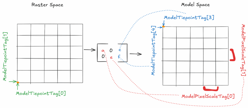
What is most notable about these two tags is that we can use them to build a simple affine transform to easily and efficiently convert between raster space and model space. Most GeoTIFF files represent projected data and use such an affine transform, which means that they only need to provide this mapping for a single point. Thus, most commonly, the ModelTiepointTag contains just one point, the array origin, and its coordinates in both raster space and model space.
Less commonly, the ModelTiepointTag tag includes multiple points, for example to provide a list of ground control points (GCPs) for some sort of non-affine transformation or warping. In this case the ModelPixelScaleTag tag would be omitted. While providing multiple GCPs is theoretically possible, no convention for what to do with multiple points is widely-supported by tooling. Moreover, the specific transformation algorithm or warping method cannot be expressed with any of the GeoTIFF tags, leaving tooling that might want to leverage this functionality reaching outside the spec.
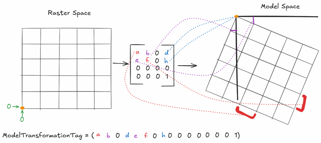
Also mentioned above is the ModelTransformationTag tag, which allows embedding an entire affine transform directly into a single tag. Conventional tooling (read: GDAL) defaults to using a tie point and pixel scale to express an affine transform, except in the case of grid rotation. A rotated grid cannot be expressed via those two tags, and as such the ModelTransformationTag tag is the only viable means of expressing such a grid.
Model space coordinate system
While the above tags give us a means of defining a grid and translating between model space, we donвҖҷt actually have any way to tie that model space to geographic space without more information. This is where the geokey tags come into play.
The GeoTIFF specification defines three geokey tags: GeoKeyDirectoryTag, GeoDoubleParamsTag, and GeoAsciiParamsTag. Exactly how these tags operate together is outside the scope of this article (but the previously-linked notebook on reading COG data does demonstrate this process in detail). In essence, together they provide the coordinate reference system (CRS) information we can use to understand the units and frame of reference for our model space as we found above. Refer to the GeoTIFF specification on “Geocoding Raster Data” for more information.
RPCs and sensor models
While NITF itself is not important to our discussion, its support for RPCs and camera models is worth mentioning, even if just in passing. In fact, RPCs are not limited to NITF, but can be used with TIFF/GeoTIFF as well.
Rational polynomial coefficients are another parametric coordinate transformation, like affine, but provide a much greater accuracy. Affine transforms approximate the model by, in effect, stating вҖңthe Earth is flat (locally) and pixels are perfect rectanglesвҖқ. They ignore terrain relief, ground curvature, lens distortion, and atmospheric refraction, but the model is simple, fast, and good enough for most things.
Where an affine is not good enough, however, the next step is to look to RPCs. They give us a parametric mapping like:
row = P1(lat, lon, height) / P2(lat, lon, height)
col = P3(lat, lon, height) / P4(lat, lon, height)
Where P1, P2, P3, and P4 are rational polynomials (typically cubic, with 20 terms each). Calculating these obviously requires many more coefficients than an affine transformation, and is more computationally intensive, but gets us a much more accurate model of the actual ground surface. ItвҖҷs no longer flat, can factor in terrain relief, and can fix some lens distortions, but still makes some assumptions and approximations regarding time-varying geometry, atmospheric effects, and the ground surface.
When RPCs are not enough, the next step is to build a rigorous camera model. Doing so requires even more information about exact satellite ephemeris and orientation, and is even more computationally intensive.
NITF, as mentioned, supports metadata conventions to express RPCs with or without a camera model. But, interestingly, if RPCs alone are sufficient, the NITF RPC metadata can be expressed in a TIFF/GeoTIFF using the non-standard (but conventionally supported) tag RPCCoefficientTag.
WeвҖҷre not going to continue discussing RPCs or camera models for the sake of brevity, but we felt we would be remiss not to mention them at all because most conversations about geospatial metadata tend to center on affine transforms or CF conventions. In this way they miss the fact that other transformations exist and are essential for low-level image processing and high-accuracy applications.
CF conventions
As mentioned, the NetCDF core spec does not describe any geospatial conventions. For that we must look to CF conventions, a separate set of specifications designed to be used with NetCDF for this purpose. They provide a standardized set of fields (units, long_name, short_name, вҖҰ) and taxonomies of canonical names for data variables. They also specify how to map from model space to domain space (where a location is on the Earth) using the grid_mapping field and a dimensionless GridMappingVariable. Unlike the affine transform provided by the GeoTIFF tags, CF conventions have no parametric mapping function from raster space to model space because CF relies on the presence of explicit coordinate variables, which are themselves arrays. As the explicit coordinate arrays handle the mapping from raster space to model space, CF only needs to provide the mapping from model space to Earth вҖ“ otherwise known as the CRS. Here is an example from the CF documentation of a Lambert Conformal GridMappingVariable:
dimensions:
  y = 228;
  x = 306;
  time = 41;

variables:
  int Lambert_Conformal;
    Lambert_Conformal:grid_mapping_name = "lambert_conformal_conic";
    Lambert_Conformal:standard_parallel = 25.0;
    Lambert_Conformal:longitude_of_central_meridian = 265.0;
    Lambert_Conformal:latitude_of_projection_origin = 25.0;
  double y(y);
    y:units = "km";
    y:long_name = "y coordinate of projection";
    y:standard_name = "projection_y_coordinate";
  double x(x);
    x:units = "km";
    x:long_name = "x coordinate of projection";
    x:standard_name = "projection_x_coordinate";
  double lat(y, x);
    lat:units = "degrees_north";
    lat:long_name = "latitude coordinate";
    lat:standard_name = "latitude";
  double lon(y, x);
    lon:units = "degrees_east";
    lon:long_name = "longitude coordinate";
    lon:standard_name = "longitude";
  int time(time);
    time:long_name = "forecast time";
    time:units = "hours since 2004-06-23T22:00:00Z";
  float Temperature(time, y, x);
    Temperature:units = "K";
    Temperature:long_name = "Temperature @ surface";
    Temperature:missing_value = 9999.0;
    Temperature:coordinates = "lat lon";
    Temperature:grid_mapping = "Lambert_Conformal";
We can also use WKT to define specific coordinate reference systems, and, importantly, we can specify which variables they apply to. That said, we always have a requirement to provide latitude and longitude coordinate arrays, even if they are 2D arrays.
Note that these coordinate arrays are a particularly interesting solution to mapping between raster space and model space, because they allow a degree of expressability that a simple affine transform, or even warping functions, cannot begin to approach. They provide radical flexibility, making irregular grids a trivial problem and allowing things like mixed resolutions, non-rectangular grids, curvilinear grids, unstructured meshes, time-varying coordinatesвҖҰthe list goes on.
They are, however, heavy. Discrete coordinate arrays mean that every single coordinate must be stored. Additionally, translations between raster space and model space may require computationally-intensive coordinate array traversal. Conversely, parametric models, like affine transforms or RPCs, are both space and computationally efficient. Like our earlier discussion about aggregating metadata to achieve computational and storage efficiency, parametric models similarly trade some level of accuracy and expressibility to gain these advantages. Coordinate arrays obviously have their uses, and really cannot be replaced where they are required, but for a simple grid they are overkill.
GeoZarr? Or geo, in Zarr!
Over the past few years the community has been working on a GeoZarr specification, but so far nothing has been formally released. This lack of ability to express geospatial metadata in a conventional way is a core reason why we stand by our statement that Zarr is not the new COG. They are apples and oranges! Zarr is to TIFF what GeoTIFF is to what? That вҖңwhatвҖқ doesnвҖҷt yet exist! (Then add on the convention in COG for performant visualization via overviewsвҖ”we know, multiscale is coming, but it isnвҖҷt here with the same support, yet). But this discrepancy might quickly be changing because that вҖңwhatвҖқ is comingвҖҰ
At the recent Zarr summit, the community arrived at a consensus around the notion of вҖңConventionsвҖқ, an idea similar to and drawing inspiration from the notion of STAC Extensions. The idea is to create a decentralized system whereby anyone can propose a Convention without any formal gatekeeping processes. The level of support by tooling will likely depend heavily on the popularity of any given Convention. Zarr stores will be able to declare the Conventions used in their metadata, such that tooling will be able to see what Conventions a dataset has via a single explicit advertisement, instead of through inspection and various heuristics. Conventions will be versioned, and will each declare a jsonschema that can be used to validate conformance to their specification.
One of the first proposed Conventions is the geo/proj convention. This Convention uses fields from the Projection STAC Extension and specifies how to define an affine transform. Downstream libraries (such as Xarray or rioxarray) will need to adopt the Convention so that they can represent coordinate information as an actualized array when reading from Zarr stores that use the geo/proj convention. This is all very new, but it is a promising path.
Where does metadata go?
WeвҖҷve now talked at length about metadata, but we have not yet addressed one common and contentious question: where should metadata be stored?
Considering our working definition of metadataвҖ”metadata is information that helps you understand how to interpret dataвҖ”itвҖҷs clear that this metadata should be in the file so readers of the file have what they need to use it. But is this the only place it should go? And what about that other type of metadata, the kind weвҖҷve dismissed up to now: the metadata that helps users find the data they need?
Well, we know we can put the usage metadata in the file, obviously, but what options do we have to store the search and discovery metadata? It should be equally obvious that we canвҖҷt store that metadata exclusively in the file. If someone knows about the file then they have already discovered it! So, where should we put that metadata?
Zarr allows data producers to define arbitrary metadata for any group and for any array. In native Zarr this metadata is stored in a json file at the top level. In the array case this means the json file sits alongside the directories of chunk data. Of course, Zarr is flexible! So one could also store metadata as another array within a group, but no conventions exist around this idea yet. The recent Zarr summit touched on the possibility of using this approach to store chunk-level metadata. Doing so is certainly possible right now, but until a convention is proposed and adopted by tools, client libraries won’t know how to interpret metadata stored in such a way.
TIFF also supports arbitrary metadata, but, as a single-file binary format, it must be embedded into the metadata via a custom tag and some appropriate encoding. We see GDAL do exactly this (recall the GDAL_METADATA tag that embeds XML-format metadata into TIFF encoded as an ASCII string). This said, with TIFF, the length of the metadata bytes cannot be known without parsing the entire metadata structure. When accessing a TIFF cloud-natively, this uncertainty can be a problem because tooling canвҖҷt definitively know how many bytes to request to ensure it gets all the metadata it needs. Bloating TIFF metadata is therefore not advised.
So, can we finally answer the question? Where should you put metadata:
- in the data format?
- outside the data format?
- both?
Generally, it’s best to think about how the metadata is intended to be used. For instance, let’s consider the case of a cloud cover percentage value, aggregated at the array level. The primary use for such a cloud cover percentage is search, as that statistic is most useful for eliminating files that cannot contain useful data. Thus, it makes sense to store that metadata value outside the data format itself, so users can assess whether a given array is of interest or not without ever touching the file.
On the other hand, metadata that is essential for decoding the array, as we said above, is clearly needed within the data format since the array data is unusable without it. Some of this kind of metadata is rather low-level and not at all useful for users except when trying to read a particular chunk of data, and therefore it doesnвҖҷt necessarily make sense to also store those values outside the format.
Yet, some metadata fields are useful both inside and outside the data format. For instance, the geographic area that the data covers is obviously something that you need to have information about when reading data, but it is also useful when searching for data. Some fields that seem primarily search-related can be useful in-file, to provide context about the data. On the other side, some seemingly low-level metadata like data type or array size can also be useful outside the format metadata, as they can provide clues to tooling how it should prepare to use the data before ever making a request to the dataset.
Sometimes the lines blur even more. It is not without precedent to want to store external metadata alongside or even in the data format to provide a canonical copy of that metadata for search services to index. And, as we look to the future, we hope weвҖҷll soon start to see better support for varying levels of metadata within raster formats all the way down to the chunk level, to support more access patterns with better efficiency via Parquet-like predicate pushdown.
So, do we have a good answer here? Well, like with all things of importance, the real answer is вҖңit dependsвҖқ. Our rules of thumb are outlined above. They generally work well, but of course we see exceptions. And, as the ecosystem and tooling shifts, we expect to see those rules evolve accordingly.
Conventions canвҖҷt just be conventional
Historically, the community has depended on many conventions in an implicit, informal way, often defined by tooling implementations and little else. But we need to move beyond that conventional understanding of conventions, and shift to something more formal and organized.
We are particularly excited about the direction the Zarr community has chosen for its Conventions because they appear to be converging on ideas weвҖҷve been discussing recently around data formats as the sole means of communicating interoperability. That is, so often in conversation we might say something like, вҖңthe file is a GeoTIFF, so tool ABC should be able to read itвҖқ or вҖңthis dataset is Zarr v3, so we have to use a newer tool version to open it.вҖқ Except thatвҖҷs not really all there is to the story, as weвҖҷve seen.
Metadata space
Data formats define the format of their internal metadata: TIFF uses its tag format, Zarr says JSON. The format specification also applies some additional constraints on the metadata. For example, any arbitrary valid JSON document is unlikely to be valid Zarr metadata. Zarr specifies that certain key fields must be present and defines the shape of their values, but it doesnвҖҷt limit the possible values for many of those fields, nor the addition of other fields. This implies an infinite space of JSON documents that represent valid Zarr metadata.
ConventionsвҖ“official in the new Zarr sense, or informal in the traditional senseвҖ“then layer on top of this metadata space and provide a narrowing of possible metadata values. In the absence of conventions, for any domain-specific application which is not expressible using just the core specifications fields, each individual combination of metadata fields and values is a separate case that tooling needs to be able to handle. ItвҖҷs an impossible task! Is the field with the CRS metadata вҖңprojвҖқ or вҖңprojectionвҖқ or вҖңcrsвҖқ or вҖңCRSвҖқ or вҖңsome-other-random-field-nameвҖқ? We canвҖҷt know. At least not without applying some convention.
Conventions steer us to a common set of “combinations” within any given data format. But, how can we know a specific convention is in use? Traditionally, through inspection and heuristics. Does it look like a file following a convention? Then maybe it is. This works well enough for certain things, like knowing if a TIFF is a GeoTIFF: does it use any GeoTIFF keys? Then it is a GeoTIFF. But what version of the GeoTIFF spec?
Moreover, what if our GeoTIFF has a value of 50000 for its Compression tag? What does that mean? That value is not in the TIFF spec. According to libtiff, it means zstandard compression. But, how do we know if the writer was using libtiff? So is it really zstandard? ВҜ\_(гғ„)_/ВҜ In the absence of formal conventions, we get informal conventions, without coordination. Tools make their own choices, and the absence of consensus undermines interoperability.
Here we see the need to both be able to define conventions in a formal way, and to advertise what conventions a specific dataset follows, so users/tooling can more easily confirm compatibility. Simply knowing the вҖңdata formatвҖқ is not necessarily enough. Heuristics are also not enough. We need to do better to make вҖңmini-formatsвҖқ: well-specified combinations of data formats and the conventions on top that make them compatible with a given set of tools in a specific domain. Additionally, we need to make conformance explicit through advertisement within the data formatвҖҳs internal metadata.
The data format and convention set is also not enough on its own. We need versions for both data formats (which we tend to have) and also for the conventions. This way tooling can describe compatible formats and convention sets in the same way code libraries describe their compatible dependencies: format_a>=1.2, convention_g>=0.7.1, convention_w~=3.4вҖҰ All of this is why hearing about the Zarr decision to do all of this with its new concept of Conventions is so exciting!
Metadata, on the surface, seems like an utterly boring topic. But, as it turns out, metadata is multifaceted and complex in some unexpectedly interesting ways. The crux of what we have been getting at over the course of this series, that the meaningful differences between raster formats are quite minimal, really comes down to metadata: what can or cannot be expressed in a formatвҖҷs metadata is the primary mechanism by which formats support differentiating features. By understanding metadata better, we can better understand the formats themselves, and we also gain a valuable perspective on how we can use metadata to shape a more efficient and interoperable future.
If you have additional thoughts on metadata, or on any of the examples or discussion topics we address in this blog series, weвҖҷd love to continue the conversation! Reach out to us on our contact us page, and check out the rest of the corresponding posts on our blog.