Sand and dust storms are a frequent occurrence in many different parts of the world and pose serious health and environmental risks, affecting everything from air quality to agricultural productivity. They are also becoming more frequent with time due to climate change, making it more important than ever to reliably detect, track, and–if possible–predict them. Earth observation satellites allow us to observe these sandstorms in near-real-time, but existing detection algorithms fall short of providing fine-grained segmentation masks and do not always distinguish between dust and other kinds of aerosols. As part of the UNDDPA Innovation Cell’s efforts towards addressing the challenges of sandstorms, we addressed this capability gap by training a deep convolutional neural network to segment sandstorms in satellite imagery using supervised machine learning. The ability to reliably segment sandstorms in satellite imagery opens up new avenues of analysis for understanding how sandstorms develop and evolve.

In this blog, we walk through our approach to the problem, evaluate the quality of our results, and compare them against some of the existing solutions. We conclude with some thoughts on how this work might be developed further. Throughout this text, we use “sandstorm”, “dust storm”, and “dust” interchangeably.

Existing sandstorm detection approaches

The use of neural networks in detecting sandstorms is, to our knowledge, under-explored. Most existing approaches use traditional techniques such as band arithmetic and RGB compositing.

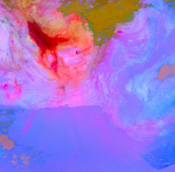
For example, a standard approach to detecting sandstorms, commonly used in meteorology, is the “Dust RGB” (Figure 1) composite available for the GOES and EUMETSAT satellites. This data product is created by compositing different bands and band-differences into an RGB image such that various phenomena like dust, ash, clouds, etc. show up in distinct colors. While useful, this approach has the limitation that the colors are not always easy to interpret and do not always correctly distinguish between dust and other kinds of aerosols.

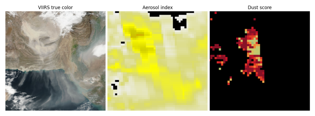
Other relevant products include the Aerosol Index and the Dust Score. As can be seen in Figure 2, these have very low-resolution, often have pixels with missing data, and are not quite dust segmentation masks.

Yet another product is the Deep Blue Aerosol Type, which does in fact provide a dust segmentation mask. However, it is not very discerning and seems to produce way too many false positives to be useful.

Our approach: sandstorm detection as a semantic segmentation task

Based on our experience solving similar problems before–most relevantly: cloud detection–we posed the problem of sandstorm detection as a semantic segmentation task where we trained a model to classify each pixel in satellite images as “dust” or “not dust”. Unlike some of the scientific data products mentioned above, this approach is not based on any scientific interpretation of the reflectance values picked up by the satellite sensor, but instead relies solely on the visual appearance of the pixels in the image. This approach is also more straightforward than the Dust RGB composite since it doesn’t require complicated color interpretations.

We expected this approach to work well based on the assumption that dust storms are usually visually distinct enough to be delineated in the image by a human, which in turn implies that a training dataset can be constructed to train a semantic segmentation model.

For those curious, we did also test the Segment Anything model on this problem (as part of the labeling process), but found its performance lacking.

Building a dataset

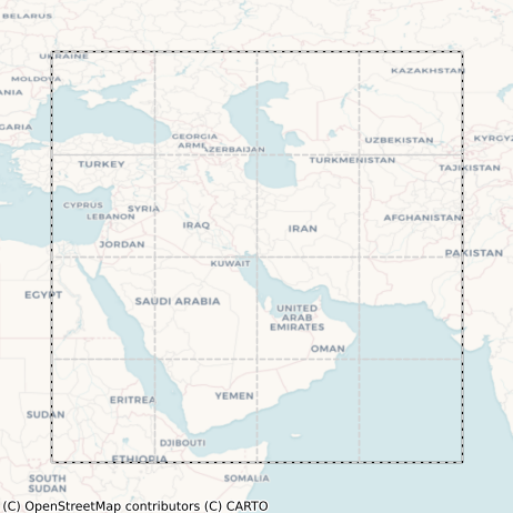
Since there is currently no existing sandstorm segmentation dataset, we had to build one from scratch. Starting from scratch meant that not only did we not have labels for sandstorms, but that we did not even have imagery with sandstorms in the first place. So the first step was to use NASA Worldview to manually find dates with sandstorm occurrences. To constrain the problem, we restricted ourselves to the spatial region shown in Figure 3 and to the time period of 2022-2023.

Imagery

For the imagery, we used imagery captured by the Visible Infrared Imaging Radiometer Suite (VIIRS) instrument on board the NASA/NOAA Suomi National Polar orbiting Partnership (Suomi NPP) satellite. This imagery is available at 1 km spatial resolution, covers the entire world, and is updated daily.

An additional wrinkle was that the normal surface reflectance data product failed to properly capture dust, especially over land, and had significant visual artifacts that could be detrimental to training a model. The corrected reflectance product (available via the GIBS API), on the other hand, captured dust much better. A comparison between the two is shown in Fig. 4. We, therefore, chose to use the corrected reflectance product.

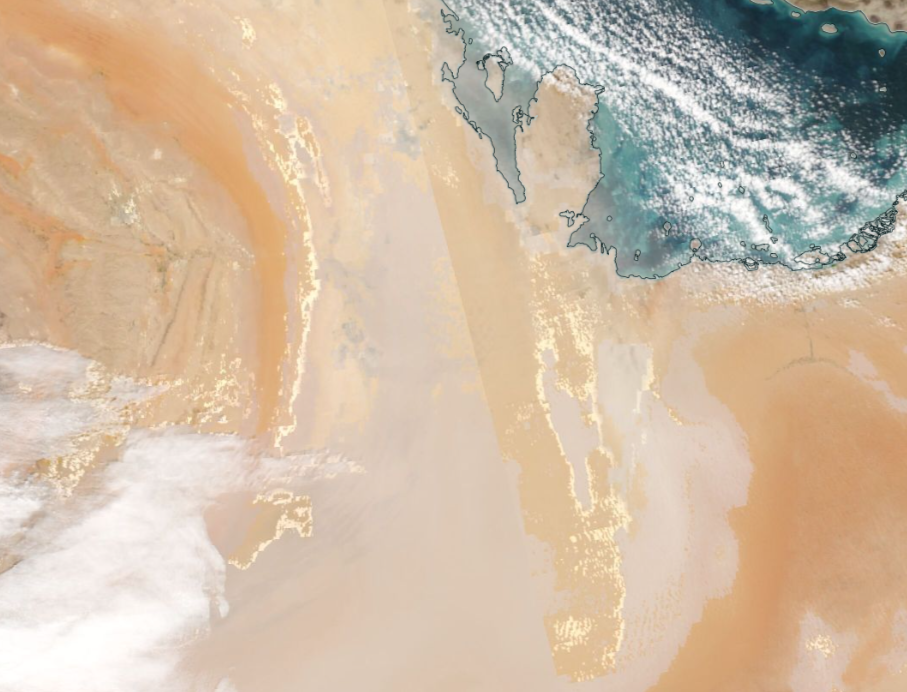
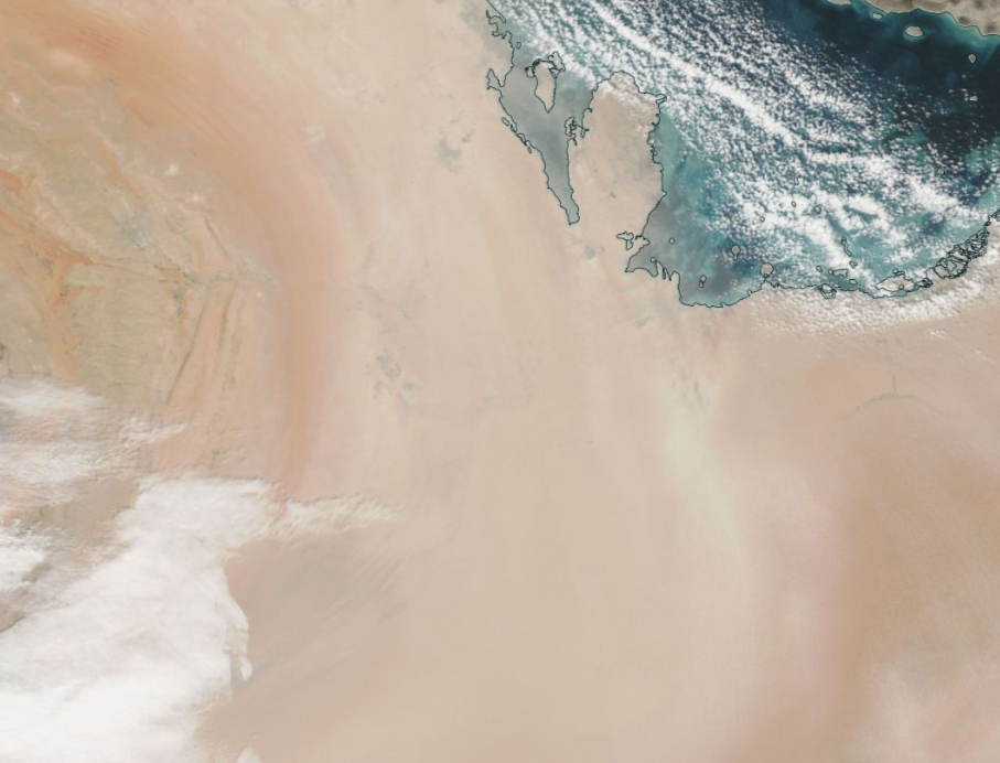
Figure 4: Difference in dust visibility between normal reflectance (left) and corrected reflectance (right). It can be seen that dust appears strangely discontinuous and riddled with visual artifacts (the bright jagged boundaries) in the normal reflectance image, whereas the corrected reflectance image has no such problems. Link to interactive comparison: https://go.nasa.gov/45kvh70.

Labeling

Data labeling is the most important and the most expensive part of any machine learning project. We used the open source labelme tool to create polygon labels for sandstorms. This turned out to be easy in some cases, such as over water, but more difficult in others, such as over desert regions, especially with less intense sandstorms (Figure 5). Other tricky instances included thin clouds (Figure 6) and even the Sun’s reflection in the water (Figure 7).

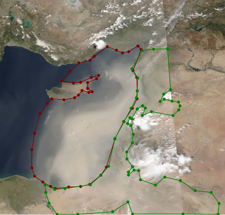
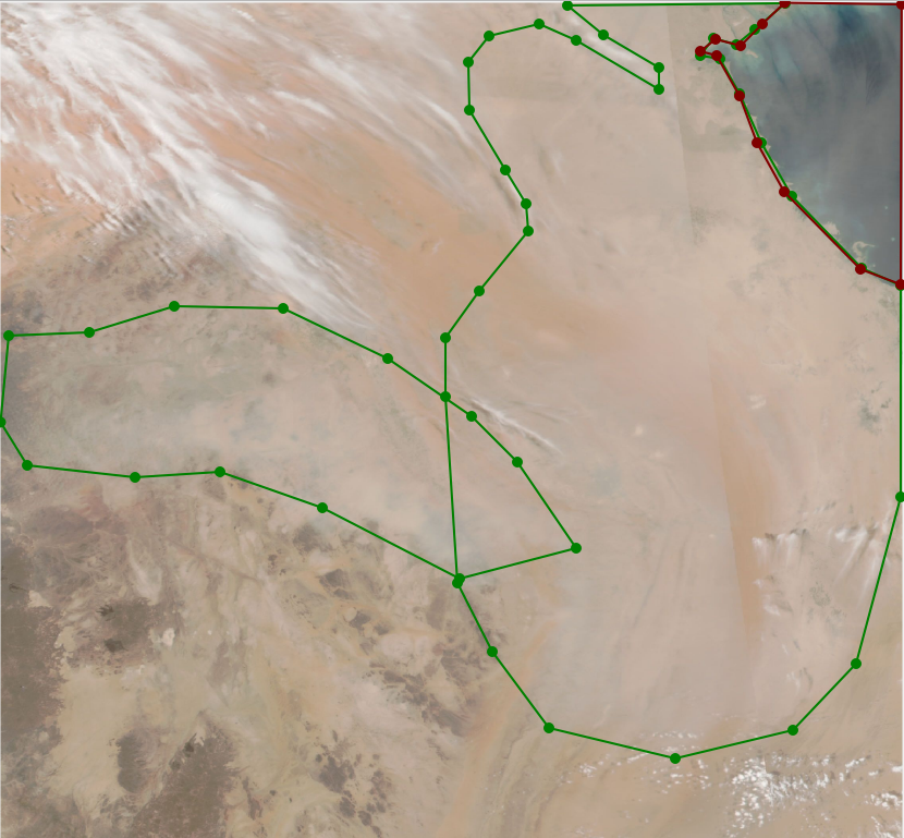
Figure 5: Sample labels from the training set. Intense sandstorms (left) were easier to label than less intense sandstorms especially over desert terrain (right).

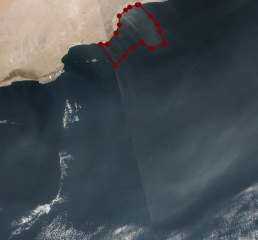
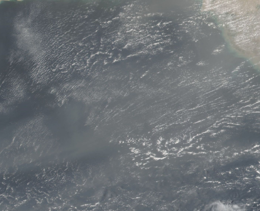
Figure 6: Tricky labeling instances: thin dust or thin clouds?

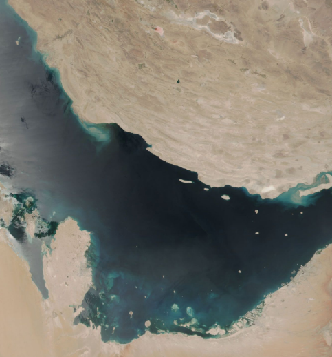
Figure 7: Tricky labeling instances: Dust or the Sun’s reflection in the water?

We ended up labeling about 500 images in total with ~85% being from 2022, constituting the training set, and the rest being from 2023 and constituting the test set. The distribution of these labels is shown in Figure 8. Given that they were not created by domain experts or even professional labelers, the labels were admittedly imperfect, but somewhat surprisingly (as we shall see below), they still allowed us to train some very high quality models.

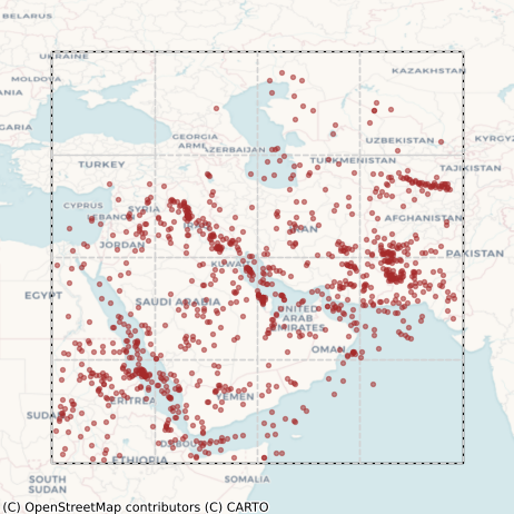
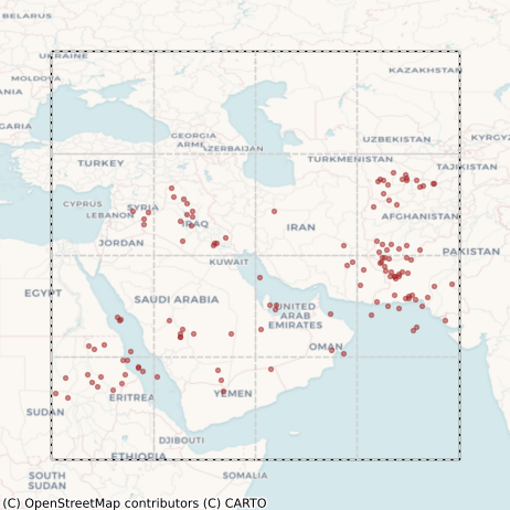
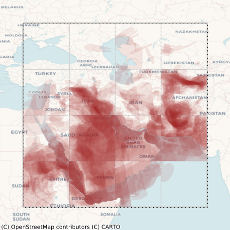
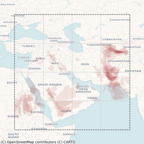
Figure 8: Distribution of labels from the training (left column) and test (right column) sets. Top row: centroids of individual polygons. Bottom row: All polygons overlaid on top of each other.

Training

We used an FPN model with a ResNet-18 backbone as our model architecture and conducted several cross-validation experiments using our open source geospatial machine learning library, Raster Vision. The experiments included various combinations of inputs in addition to the true color RGB imagery, such as additional VIIRS bands, aerosol index, and even the Blue Marble imagery. The idea with the last of these was to see if the model could learn to do a kind of implicit change detection by comparing against a completely clear image.

Results on the test set

We omit a detailed breakdown of the cross-validation metrics here and instead just present the test set metrics. To compare models, we used the F1 score metric, which is a combination of recall (of all the dust pixels present, how many did the model find?) and precision (of all the pixels the model classified as dust, how many were actually dust?). The best performing model turned out to be one that took in 5 additional VIIRS bands (M11, I2, I1, M3, I3) plus the Blue Marble imagery, with an F1 score of 0.800. However, the difference between this and the baseline RGB-only model (F1 score of 0.796) was not significant. 

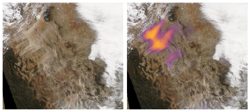
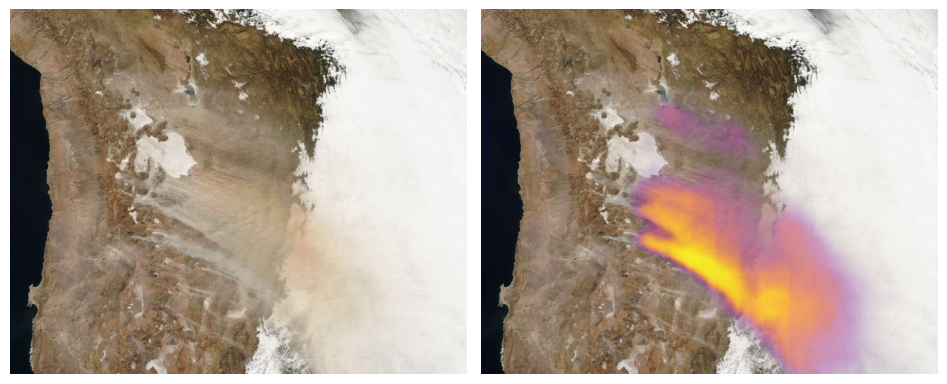
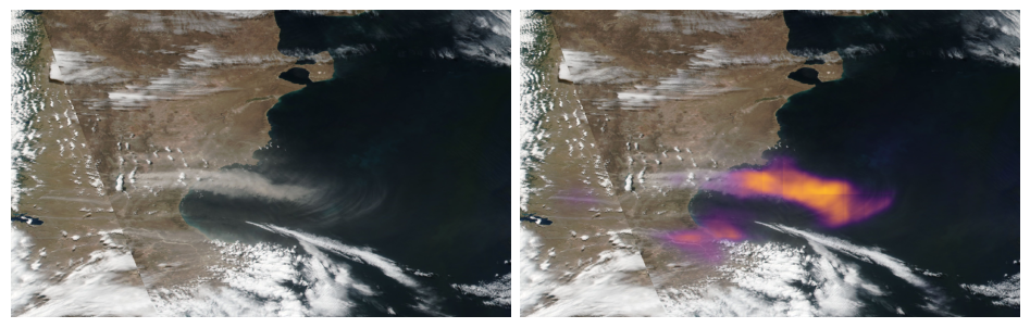
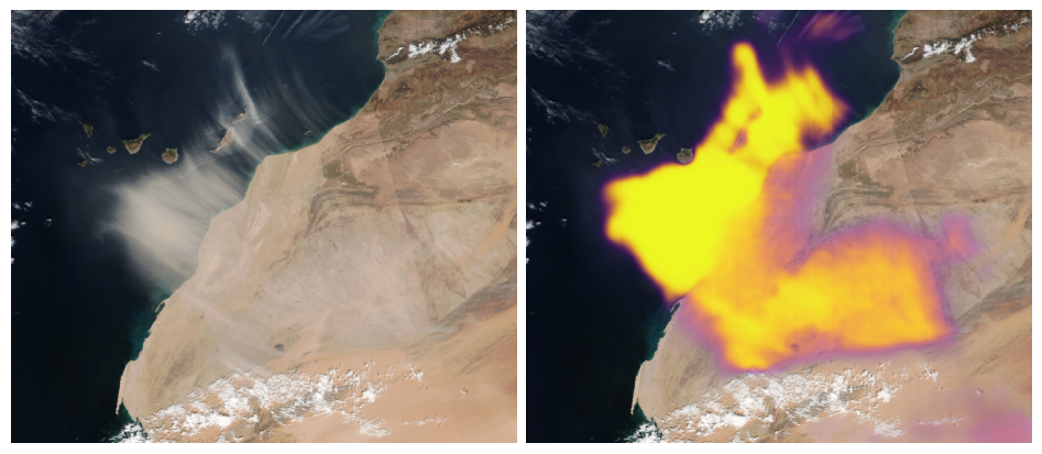
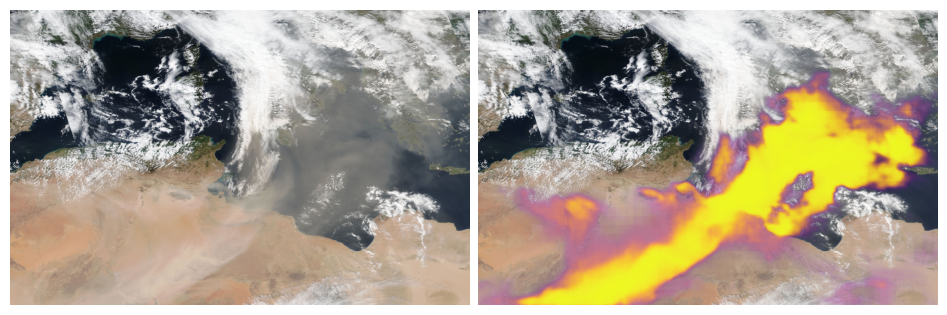
Below we present some of the predictions of the best-performing model on images from the test set. We note that these are more-or-less representative of the usual quality of the model’s predictions.

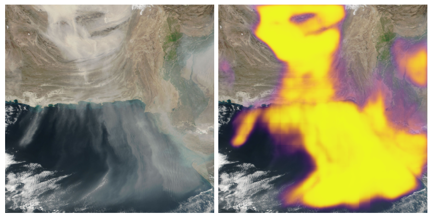
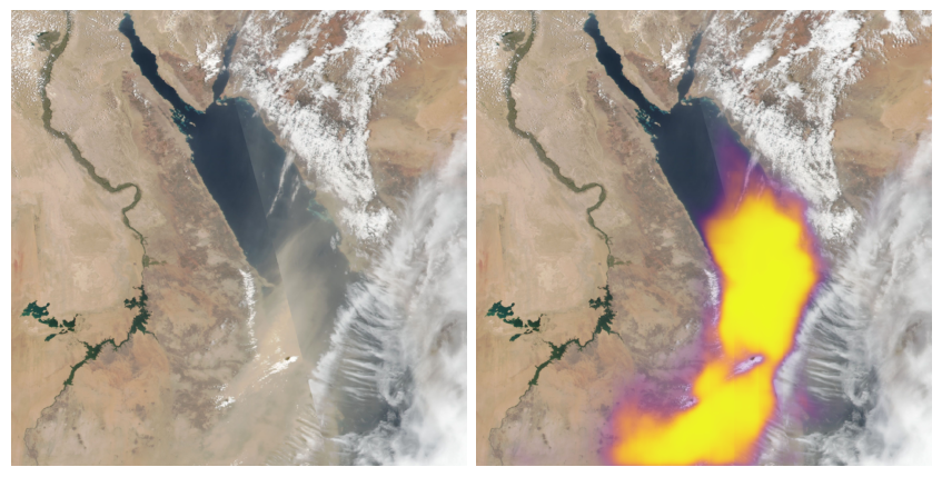
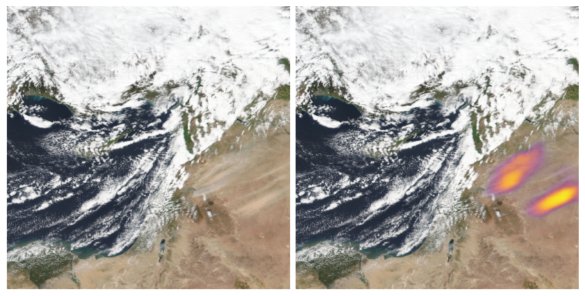
FIgure 9: Prediction on images from the test set. Left: input images. Right: the model’s predicted probability of dust overlaid on the input image.

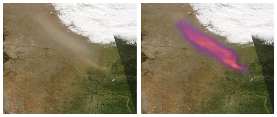
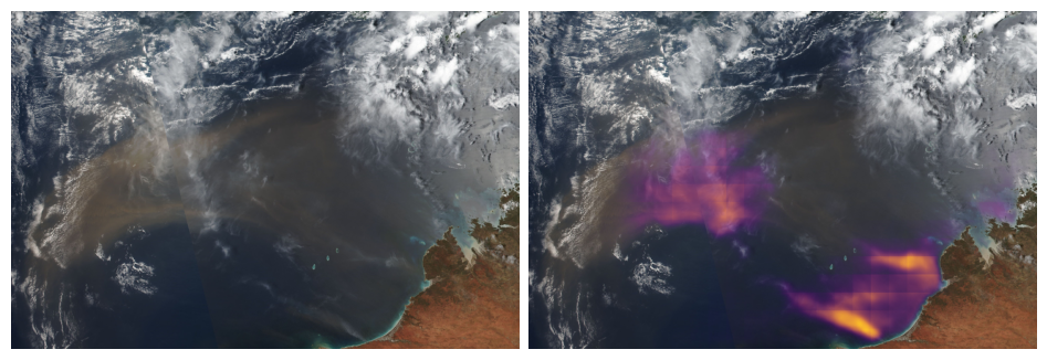
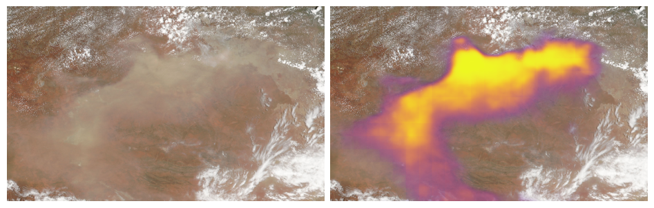
Generalization across regions, times, and sensors

We also extensively tested the generalization of our model to data outside its training distribution. This included imagery from other parts of the world, from different years (going as far back as 2010), and even from a different sensor (MODIS). The results are shown below. Note that for MODIS images, we used the RGB-only model.

Concluding thoughts

We have shown the feasibility of training a highly performant convolutional neural network model for segmenting sandstorms in satellite imagery with relatively little labeling effort. Unlike the Dust RGB composite, this model’s outputs are segmentation/probability maps that require no complicated interpretation of colors. It is also remarkably good at distinguishing dust from clouds. Such a model not only allows us to generate high-quality global sandstorm segmentation masks, but it also enables analyses of the frequency, shapes, and trajectories of sandstorms. And, since it works on imagery from any time period, these analyses can be extended backwards in time to as far back as 2002 (earliest MODIS imagery). Furthermore, the model can be iteratively improved by expanding its training dataset to include more examples to address any shortcomings.

While this model is currently limited to VIIRS and MODIS (and thus to a temporal resolution of one day), we can also easily take this overall approach and apply it to train a similar model on imagery from geostationary satellites such as GOES and EUMETSAT, which will allow us to produce high-quality dust segmentation maps every 15 minutes! This will be useful for detecting more short-lived sandstorms and might aid in forecasting.

What’s next?

As climate change intensifies, the ability to quickly detect change at a detailed level becomes more and more impactful. Leveraging machine learning gets better data into the hands of scientists so they can respond faster, rather than spending their time manually labeling datasets. 

At Element 84, we are passionate about leveraging our skill sets in geospatial AI and ML to address climate change. Many problems in remote sensing that have traditionally been solved via simple band arithmetic and pixel-wise methods can benefit from upgrading to a more modern approach based on deep learning and we have a track record of doing just that. In addition to detecting sandstorms, we have previously built ML solutions for detecting tree canopy cover, tree health, floods, and even clouds, and are currently collaborating with American Water on detecting algal blooms. If you have a problem that you’d like to discuss in-depth with our team, please get in touch! We also believe strongly in open source–all the ML training described in this blog was carried out using our open source Raster Vision library.