In this blog, we discuss our experience using Kerchunk to improve access times to short-range streamflow predictions generated by NOAA’s National Water Model Predictions Dataset, achieving a speedup of 4 times, using 16 times less memory.

What’s challenging about climate data analysis today? 

Near real-time analysis of climate data requires efficient access techniques that are easy to use and quick enough to answer pressing concerns. In the best case, the climate data is available in a cloud-optimized data format which can easily be accessed remotely. However, often the data is only available in a more traditional format, such as NetCDF, which is widely used in the climate sciences due to its easy packaging of multi-dimensional data. Unfortunately, it is not cloud optimized, thus requires downloading the entire dataset before it can be analyzed, which impedes getting quick answers.

One such dataset is NOAA’s National Water Model Predictions Dataset, which contains short, medium, and long range predictions of various stream metrics, including streamflow, for more than 2.7 million streams in the continental United States. This predicted streamflow can be useful for forecasting flood risk, especially in areas that don’t have more detailed, local stream models available. The quicker we can assess flood risk, the better we can prepare our communities and minimize damage. However, since the NetCDF data is not cloud optimized, analyzing the streamflow for an area of interest even just a few hundred square miles is a time consuming endeavor.

Who does this data accessibility work benefit?

Researchers need to give decision makers relevant and accurate information so they can make the most useful decisions for flood risk mitigation. Given that recency and speed of data access are paramount for this, what transformations can we apply to the NWM Predictions Dataset to make this easier? Let’s take a look.

Improving on existing tools for data access

The two main techniques for optimizing data access in computer science are deferring and minimizing: we should defer fetching data as long as possible, and, when we must, we should fetch as little data as we can to do what we need. Cloud optimized data formats exploit these techniques to great effect. Zarr allows cloud optimized access to multi-dimensional data. Parquet, better suited for tabular data, is also an option. We’ve previously benchmarked various Zarr and Parquet encodings of the NWM Retrospective Dataset, and found that rechunking the Zarr dataset along the time dimension improves performance for time based queries. Using the rechunked dataset, we can answer questions like, “What was the average streamflow per week of every stream in this area?” much faster.

Creating such a chunked Zarr dataset from the original NetCDF is a computationally and spatially expensive process. Not only does it take a while to ingest the NetCDF data and convert it into a chunked Zarr file, it takes almost as much space to save as the original NetCDF dataset. This is worthwhile for the Retrospective Dataset, a static dataset which is no longer written to, but which will be read many times by researchers performing historical analysis. However, for the Predictions Dataset, which is written frequently and where recency is of great value, such processing is prohibitively expensive for researchers interested in small areas of interest, and has the potential to delay analysis and flood risk mitigation.

What we need is an index. Generating a map into the NetCDF file would allow us to navigate it similarly to Zarr. Kerchunk does exactly that: it generates a JSON index file which can be used by the xarray library to read the dataset using the Zarr engine. This JSON file is lightweight and can be created quickly. Using this file, the NetCDF data can be accessed in a more cloud optimized manner, significantly speeding up analysis.

Prediction data in the National Water Model 

For this work we focused on the short range predictions in the NWM Predictions Dataset. Every hour, the NWM generates predictions for the next 18 hours, all as individual NetCDF files:

$ aws s3 ls s3://noaa-nwm-pds/nwm.20230312/short_range/ | grep channel_rt | wc -l

432

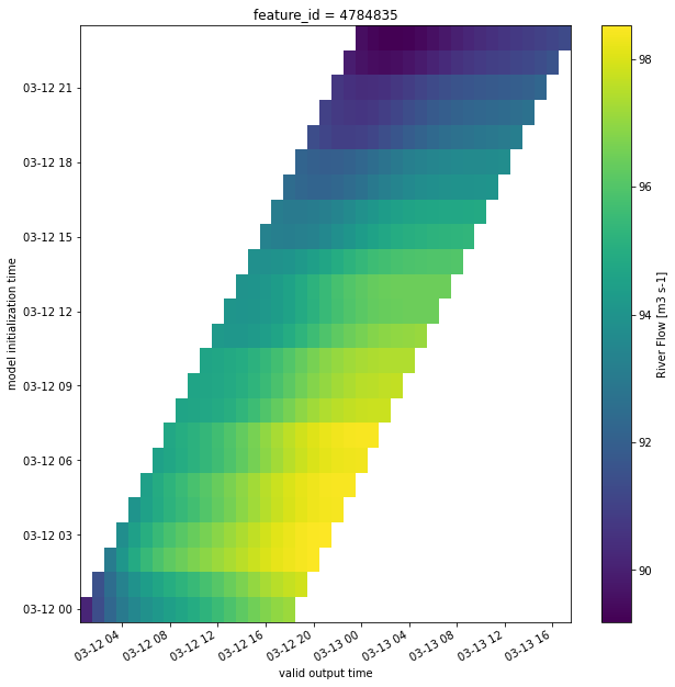
Each of these files is about ~12.3MB, making the predictions about ~5.3GB per day. Each of these files contains predictions for each of the 2.7 million streams in the continental United States. If we visualize the predictions for just one of these streams, it looks like this:

Benchmarking cloud-optimized data formats for data access

To benchmark the performance of various formats, we created a Jupyter Notebook with a sample analysis. In the notebook we fetch data for the Lower Schuylkill HUC-10, an area of interest of about 698 km². Then, for each stream within it, we calculated the mean deviation of streamflow prediction. Variation in streamflow is an important signal for judging confidence in the predictions.

The initial notebook read the raw NetCDF data as provided by the NWM Predictions Dataset, and provided baseline performance. Next, we converted the NetCDF data into Zarr files and redid the experiment with those. Then, we created Kerchunk index files for the NetCDF data, and redid the experiment with those. Finally, we created a Kerchunk metaindex which combined all the individual Kerchunk indices, and redid the experiment with that.

Kerchunk Combined is the fastest data access format 

The notebooks were executed on our JupyterHub installation that ran on r5.xlarge pods on Kubernetes running on AWS. They had 4 CPU cores, 32GB of RAM, and proximity to S3 buckets for fast data access. The full results can be seen on GitHub. Here we highlight some key takeaways:

We observed that the performance of the Kerchunk Combined metaindex was the highest, running more than 4 times faster than accessing the native NetCDF file. If we break this down, we observe that most of the time spent in the first three cases is in fetching and subsetting the data. Once it is available in memory, calculations run instantly. On the other hand, with the Kerchunk Combined metaindex, data is accessed lazily, fetching just the data needed once a calculation is triggered:

However, those instantaneous calculations in the first three cases come at a high memory utilization cost:

In our experiments we observed the Kerchunk Combined approach used 16 times less memory than raw NetCDF access.

What’s the difference between cloud-optimized data formats for data access? 

How is this happening? And why is there such a marked difference between using the Kerchunk index and the Kerchunk Combined metaindex? The key difference here is the method we use to open the dataset in xarray. In the first three experiments, namely NetCDF, Zarr, and individual Kerchunk, we use xarray’s open_mfdataset method that allows reading a multi-file dataset. Unfortunately, for xarray to create an internal representation for data traversal, it must read all the files in the multi-file dataset:

fs = s3fs.S3FileSystem(anon=True)

date = '20230312'

netcdf_url = f's3://noaa-nwm-pds/nwm.{date}/short_range/nwm.t*z.short_range.channel_rt.*.conus.nc'

fileset = [fs.open(file) for file in fs.glob(netcdf_url)]

ds = xr.open_mfdataset(
    fileset, engine='h5netcdf', data_vars=['streamflow'],
    coords='minimal', compat='override',
    drop_variables=[
        'nudge', 'velocity', 'qSfcLatRunoff',
        'qBucket', 'qBtmVertRunoff'])

In the fourth experiment using Kerchunk Combined, we use xarray’s open_dataset method with the Zarr driver specified. This allows xarray to defer reading the file until needed, and index file allows the Zarr driver to efficiently access the relevant pieces:

fs = s3fs.S3FileSystem()

date = '20230312'

kerchunk_url = f's3://azavea-noaa-hydro-data/noaa-nwm-pds/nwm.{date}/short_range/nwm.short_range.channel_rt.conus.json'

with fs.open(kerchunk_url) as f:
    kerchunk = fsspec.get_mapper(
        'reference://',
        fo=json.load(f),
        remote_protocol='s3',
        remote_options={'anon': True})

ds = xr.open_dataset(kerchunk, engine='zarr')

By deferring the data fetching to later in the workflow (using open_dataset rather than open_mfdataset), and fetching only the data we need (using the Kerchunk Combined metaindex), we significantly improve data access speeds and resource utilization for the NWM Predictions Dataset. This demonstrates how this important dataset can be used to efficiently answer questions about predicted streamflow and assist with flood risk mitigation.

Limitations of Kerchunk

The biggest limitation of this approach is the high data transfer requirement, whose amount doesn’t change significantly between the raw NetCDF (~2.14GB) and the Kerchunk Combined (~1.74GB) approach. This is because the raw NetCDF data is published as 18 slices every hour of short range prediction data, each the size of the entire continental United States, totalling 432 files per day. When indexed via Kerchunk, we mirror the existing scheme, which is chunked along the time dimension. For spatial queries, which subselect the streams within a certain area, we would have to rechunk the dataset every hour as new predictions are added, which would take longer and cost us the recency of data. Since the data transfer is on the same order of magnitude as the raw files and the RAM usage and time taken is much faster, this technique is still a valuable improvement.

Another limitation of Kerchunk is that sometimes the generated index itself can be prohibitively large, and can take a long time to parse. In this case, the index for a full day’s short range predictions is about ~5.3MB, which is quite manageable. Since short range predictions are only stored for a month, and older data is rotated out, this index will never be larger than ~160MB, which can easily fit in memory.

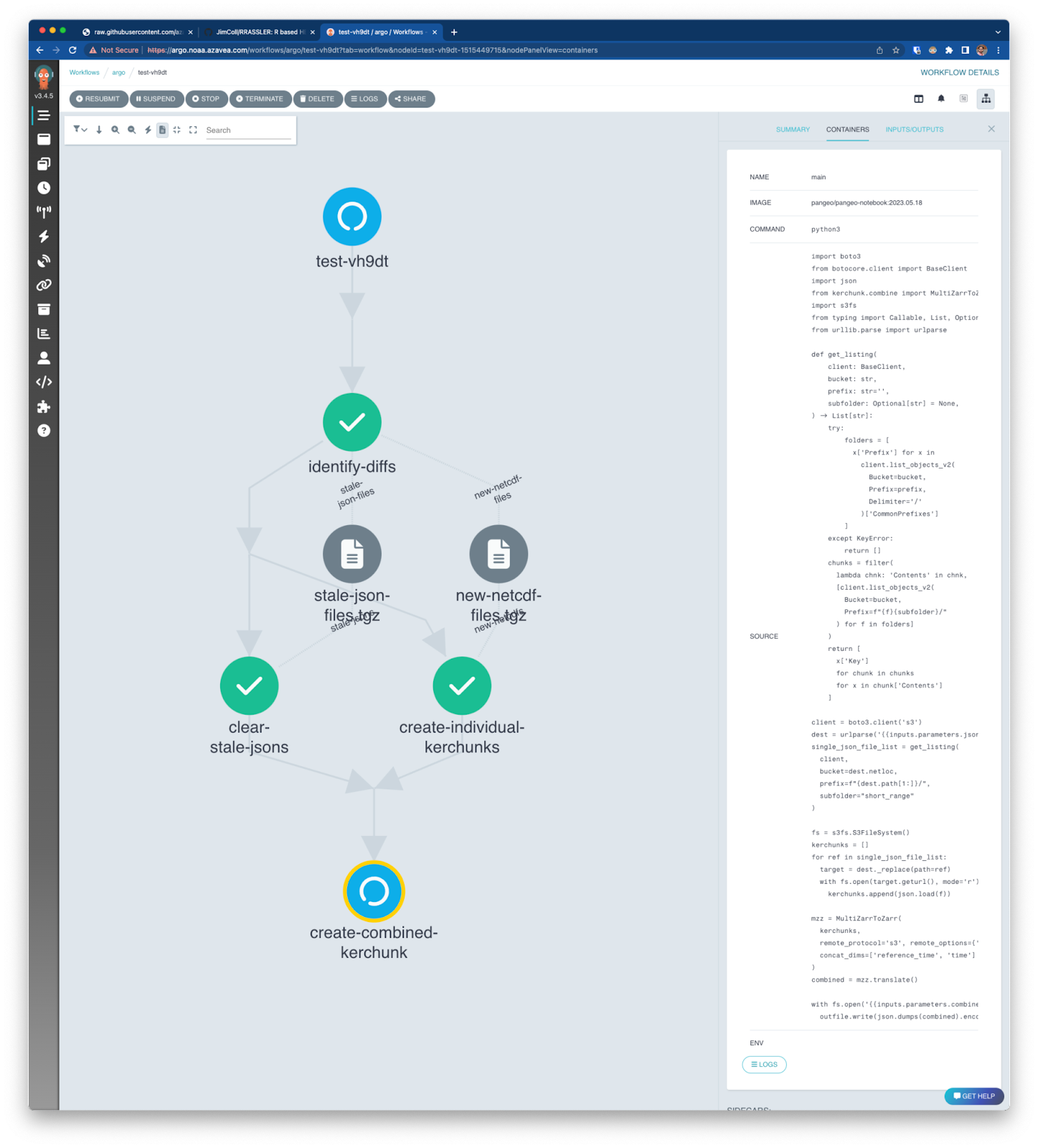
Creating a Kerchunk Combined Argo Workflow to facilitate data access

Now that we’ve verified that the Kerchunk Combined approach offers best performance, let’s sketch out an operationalized workflow. Since the short range predictions are published every hour, we need something that reads the new predictions, adds it to an existing index and removes references to old files that no longer exist. We used Argo Workflows for this, which allows the creation of dynamic workflows on demand. The workflows are available on GitHub, and ran for more than 3 months, making a Kerchunk index available for general use. We also published a version of the above experiment notebook that used the workflow-generated Kerchunk Combined index.

As the funding for this project ended, those workflows are no longer actively executing. The most recent version of the Kerchunk index is available here: https://element84-noaa-nwm.s3.amazonaws.com/public/nwm-combined-kerchunk.json. Those workflows can be deployed by anyone to their Argo Workflows instance to continue generating current versions of the index.

This Kerchunk Combined index points to copies of the prediction NetCDF files from July 26 to August 24, 2023, available in the same bucket, so that it can continue to be used as a reference after the ephemeral predictions are gone from the NWM PDS bucket. A demonstration of how to consume this file can be seen in this version of the above experiment notebook that uses the Argo workflow generated Kerchunk Combined index.

Acknowledgements

This work was done under NOAA SBIR NA21OAR0210293. We thank our subject matter experts Fernando Aristizabal, Sudhir Shrestha, Jason Regina, Seth Lawler, and Mike Johnson. I also thank the entire Element 84 project team for all their effort, ingenuity, and perseverance: Eliza Wallace, Justin Polchlopek, and Stephanie Thome.