The stactools Raster Footprint Utility

Every STAC Item contains a geometry attribute that defines the geospatial extent of the data described by the Item. For raster data, the geometry attribute is one or more polygons that enclose the raster pixels, i.e., a raster footprint. Generating accurate raster footprints is often a non-trivial task, leading to the recent development of a raster footprint utility in the stactools Python library. However, some familiarity with the challenges encountered when creating raster footprints, and the corresponding options available to address them, is necessary in order to use the raster footprint utility effectively. This blog post aims to provide that familiarity, enabling the reader to create accurate raster footprints for use in their STAC metadata.

Raster footprints

The projection problem

At first glance, creating a raster footprint seems like a straightforward task. Raster data is inherently rectangular, so a polygon with a vertex at each corner of the raster grid should be sufficient. Using an ESA WorldCover tile as an example, we see that it is cleanly bounded by a simple four-vertex polygon:

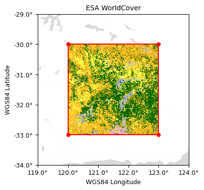
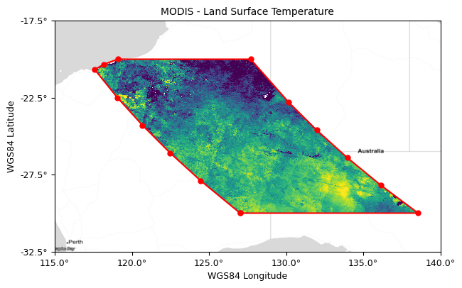
Case closed, right? Not quite! We “cheated” in the above example. The native coordinate reference system (CRS) of the ESA WorldCover image is the geographic WGS84 (EPSG:4326) system. This is the same CRS required by the geometry attribute in a STAC Item, meaning the raster data and our minimal raster footprint polygon naturally align in this case. Most remote sensing data, however, is stored in a projected CRS and is therefore distorted with respect to WGS84. A better example is a MODIS raster tile, which uses a sinusoidal projection. When viewed in WGS84, we see that a polygon defined by the four corners of the raster grid, which is highly distorted in the WGS84 CRS, isn’t quite up to the task:

We have a gap on the east and gore on the west. Not great, and it’s not just aesthetics at play here. These inaccuracies are relevant to downstream applications that work with STAC Items, e.g., STAC APIs that respond to queries for Items within a defined polygon or bounding box. Discrepancies between Item geometry attributes and actual data extents will result in spurious or missing Items in API responses.

More than a grid boundary

In addition to tightly bounding the raster grid extents in the WGS84 CRS, it may be desirable to exclude regions of the raster that do not contain meaningful information, e.g., the small region of open ocean in the northwest corner of our example MODIS image, which happens to be a land surface temperature product. Raster pixels that do not contain meaningful data are assigned a constant value, typically termed the “no-data” or “fill” value. We’d like an option to exclude regions of these no-data pixels from a raster footprint.

We also want to balance footprint accuracy versus complexity. Perfect accuracy can require (up to) a vertex at every pixel corner, resulting in polygons with huge lists of vertex coordinates. When dealing with millions of STAC Items, large footprints cause storage bloat and risk degrading spatial query performance when retrieving Items from a database. Because of this, we’d like to have options to tune this tradeoff between accuracy and complexity.

The objective

An ideal tool will generate raster footprint polygons in the WGS84 CRS that tightly bound raster pixels containing valid data, regardless of the raster’s native CRS, and provide options to balance the final footprint’s accuracy versus complexity.

The stactools approach

At a high level, the stactools approach to generating a raster footprint is to extract a polygon surrounding the valid data in the raster’s native CRS and then to transform (aka reproject) that polygon to the required WGS84 CRS. This is in contrast to transforming the raster data to WGS84 first, and then extracting a footprint. We’ll discuss why stactools does not use this latter approach when we wrap up this blog post.

If we look a bit closer by examining the implementation in the source code, we see there are four core steps:

1. Extract a polygon surrounding the valid data in the raster’s native CRS.
2. Densify the polygon with additional vertices.
3. Reproject the densified polygon from the raster’s native CRS to WGS84.
4. Simplify the densified, reprojected polygon.

Densifying the polygon refers to inserting new vertices between existing ones. This is done prior to reprojection to increase the footprint accuracy by better capturing projection distortion, which causes straight lines to become curved. Once projected, however, there may be more vertices than necessary to maintain a desired accuracy, i.e., the footprint is too complex. This is handled by applying a simplification process that removes as many polygon vertices as possible, while maintaining a maximum allowable error tolerance between the initial and simplified polygons.

To make these concepts clearer, we’ll work through each step of the process along with the options that are available to tune the footprint characteristics. We’ll produce images as we go to illustrate the effect of the options, using the same MODIS tile shown in Figure 2 as our example. But before we get started, let’s add a bit of context regarding implementation. The minimum signature to generate a stactools raster footprint is:

footprint = RasterFootprint(
    data_array,
    crs,
    transform
).footprint()

where data_array is a NumPy array of raster data, crs is the coordinate reference system in a form understood by rasterio, and transform is an Affine matrix for converting image space coordinates to geospatial coordinates. We’ll cover the raster footprint API in more detail in the next section – for now, just understand that any options we discuss are passed as additional arguments when initializing the RasterFootprint class.

OK, enough background information. Let’s dive in!

Step 1: Polygon extraction

Footprint polygon extraction is centered on rasterio’s features.shapes function, which returns a polygon and pixel value for each connected region of pixels having a common value. Since we are only interested in polygons that enclose regions of valid data (we don’t care what the actual data values are), we feed features.shapes a binary mask created from the raster data. All valid data pixels are assigned a value of one and no-data pixels assigned a value of zero in the mask. The set of polygons with a corresponding pixel value of one are retained.

If a single polygon is retained, extraction is finished. However, raster data often contains many isolated regions of valid data, e.g., islands along the coast in our example MODIS tile. This has the potential to produce large numbers of small polygons, greatly increasing the number of retained polygons and the complexity of the ultimate raster footprint. To avoid this complexity, a convex hull is applied to the shape extraction results if more than one polygon is retained after shape extraction.

Options:

• no_data: Any pixels with this value will be set to zero during mask creation. The default value is None, in which case a mask array of all ones is created, resulting in a footprint for the entire raster grid. This is the footprint shown in Figure 2. When we use a no_data value of zero for our MODIS tile, the resulting footprint now clips off the small area of ocean in the northwest corner of the tile:

Step 2: Densification

Reprojecting spatial data from one CRS to another introduces distortion. The MODIS examples in Figures 2 and 3 illustrate that if the footprint polygon vertices are widely spaced, the distortion is not adequately captured. We can improve the situation by adding new vertices to the polygon prior to reprojection. The polygons can be densified either by factor or by distance (mutually exclusive).

Options:

• densification_factor: The factor by which to increase point density within the footprint polygon before reprojection to WGS84. For example, a factor of two would double the density of points by placing one new point between each existing pair of points. In the MODIS example below a factor of three was used, which places two new points between each existing pair of points:

• densification_distance: The distance, in the linear unit of the raster’s native CRS, by which to increase point density within the footprint polygon before reprojection to WGS84. For example, if the distance is set to two meters and the length between a pair of points is six meters, two new points would be created along the segment, each two meters apart. We’ll use a spacing of 200,000 meters for our MODIS example. Notice how there is no longer a cluster of points in the northwest corner when densifying by distance::

Step 3: Reprojection

Reprojection is the transformation of the densified footprint polygon from the raster’s native CRS to WGS84. The raster footprint utility uses rasterio’s transform_geom function for reprojection. The raster data and polygons shown in Figures 1-5 are all reprojected, hence the distortion in the MODIS raster data (Figures 2-5). The MODIS raster data is a perfect rectangle when viewed in its native sinusoidal projection.

Option:

• precision: An integer value that sets the number of decimal places reported in the vertex coordinates of the returned raster footprint polygon. This does not influence the result other than to limit the implied coordinate precision to a reasonable number of decimal places.

Step 4: Simplification

If projection distortion is low and/or the footprint polygon was heavily densified prior to reprojection, the reprojected polygon will likely contain more vertices than desired. This complexity is balanced by removing vertices such that any removed vertex will be within a defined error threshold (tolerance) distance to the simplified polygon. Under the hood, the Douglas-Peucker algorithm is used for the simplification.

Options:

• simplify_tolerance: The distance, in WGS84 degrees, within which all vertices of the original polygon will be to the simplified polygon. A good rule of thumb is to use 1/2 the ground pixel width (converted to decimal degrees), but this will depend on the amount of projection distortion. Here we use a coarser value of five times the ground pixel width (about 0.05 degrees) for illustration purposes. Notice how the redundant points along the straight portions of the north and south lines have all been removed:

The raster footprint polygon is now complete. In comparison to the polygon formed from the four corners of the raster grid, illustrated in Figure 2, we have improved the accuracy by densifying the unprojected polygon with additional vertices to capture projection distortion, and decreased complexity by removing vertices that are unnecessary to meet a chosen error tolerance. We were also able to exclude the region of no-data pixels over the ocean in the northwest corner of the raster grid, thereby limiting the final raster footprint to the area of valid data.

Implementation

The raster footprints shown in above examples were created by instantiating the stactools RasterFootprint class and calling the footprint() method on the instance. For example, the MODIS footprint shown in Figure 6 was created with:

footprint = RasterFootprint(
    data_array,
    crs,
    transform,
    nodata=0,
    densification_distance=200000,
    simplify_tolerance=0.05
).footprint()

Alternative constructors

In practice, it is usually more convenient to use one of RasterFootprint‘s alternative constructors, bypassing the need to separately obtain and provide the data_array, crs, and transform arguments. Two alternative constructors are provided:

• from_href: Creates a class instance from a path or URL to a raster file.
• from_rasterio_dataset_reader: Creates a class instance from a rasterio open dataset object, e.g., from the src object created by src = rasterio.open(href).

You can also directly update the geometry attribute of a STAC Item to use a raster footprint by passing the Item and a list of one or more of the Item’s asset names to the update_geometry_from_asset_footprint method. The Item geometry is updated with the first successful footprint generated from the provided list of asset names. Finally, the data_footprint_for_data_assets method also accepts a STAC Item and a list of asset names, but produces an iterator over the same asset names along with their corresponding footprints. Check out the raster footprint module’s documentation and source code for more details.

Class inheritance

The RasterFootprint class can also be subclassed to override the individual methods that implement each step of the stactools approach for a custom implementation. In fact, if you use the raster footprint utility with MODIS data, you’ll find that footprint polygons that abut the edge of the projection may contain spurious vertices. We didn’t experience this in the examples in this post because our example MODIS tile is well within the projection extents. The MODIS stactools package contains a custom SinusoidalFootprint class that inherits from RasterFootprint. The subclass overrides the reproject_polygon method to ensure clean polygons along the projection edges.

History and future

The approach not taken

When summarizing the stactools approach for creating a raster footprint, we promised a bit more information on why stactools does not use an alternate – and potentially simpler – approach: reproject the raster data to WGS84 first and then extract a footprint outlining the data, thereby bypassing the need for densification. There are several reasons why the stactools raster footprint utility did not take this approach:

• Raster reprojection is computationally expensive.
• Raster reprojection creates a new grid of pixels which can introduce small (sub-pixel) changes to the data extents.
• In keeping with the desire for simple footprints, the stactools approach uses a convex hull to produce a single polygon footprint in instances where shape extraction produces multiple polygons. Referring back to the MODIS example in Figures 2 and 3, we see that applying a convex hull to the raster data in the WGS84 CRS would result in a gap on the east side, which is something we are deliberately trying to avoid.

That said, we’d be interested to learn about your experience if you’ve implemented an alternate approach to creating raster footprint polygons.

Enhancing the raster footprint utility

Writing this post and creating the visuals has been instructive. In addition to finding and fixing a bug or two, I kept a running list of potential improvements. All are opinions, but two of them stand out enough that I believe other users will have similar observations.

1. Specifying the distance for the simplify_tolerance option in the linear unit of geographic degrees is unintuitive. It would be great if we could use the raster’s native linear unit, e.g., meters or feet.
2. I’d like to be able to turn off the convex hull operation. There are some datasets where multiple regions of valid data exist in many product tiles, but the regions are few in number and simple in shape (ESA WorldCover comes to mind). In these cases, using a multi-polygon for the Item geometry would not introduce much additional complexity and would better describe the regions of valid raster data.

Wrapping up, stactools is just one library in a broader free and open-source STAC ecosystem. Although certainly not the only resource, the stac-utils GitHub organization is a good starting point when looking for STAC-related tools. If you have an idea for a new feature or find a bug in the stactools raster footprint utility, please open an issue in the stactools GitHub repository! We’d love to collaborate with you in building and improving the STAC ecosystem.