E84 Lab Notes: Machine Learning with SageMaker

In a previous post we showed how the E84 R&D team used RoboSat by Mapbox to prepare training data, train a machine learning model, and run predictions on new satellite imagery. In this example, we’re going to use the same imagery source and label data as a proxy for data produced by our AWS disaster response pipeline but apply a different machine learning model using SageMaker.

Machine Learning in Disaster Response

Our disaster response data pipeline is built on top of the AWS ecosystem and automates each step in mobilizing data and infrastructure in response to a disaster.

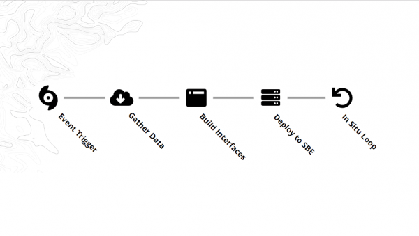
An example scenario:

1. An Event Trigger is received from a NOAA or National Weather Service alert.
2. OpenStreetMap data and satellite imagery are pulled for the affected region to be used for training our ML model to identify building locations.
3. The user interface is built on top of provisioned service AMIs (OpenDAP, MapServer, etc.).
4. A Snowball Edge is provisioned and deployed to the disaster zone.

Deployed teams now have data, network storage, and compute at their disposal. They can collect and process in-situ data, add that to a machine learning dataset, and retrain and tune the model as necessary. Once the model’s quality is deemed acceptable the response team can coordinate efforts based on predicted population centers, likely areas heavily impacted by power outages, or any other context-specific requirements.

The full architecture looks something like this:

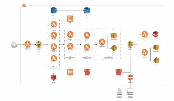
We will be exploring two pipelines that could be used to prepare the disaster metadata collection and make predictions in the field.

Although we will be using Mapbox data in the following example, aerial or satellite imagery such as Sentinel-1 and Landsat are also options.

RoboSat recap

In our previous exploration of Mapbox’s RoboSat machine learning pipeline we highlighted several takeaways after using the tool:

• RoboSat provides an end-to-end machine learning workflow, tailored to satellite and aerial imagery. Everything is covered from downloading the training imagery, preparing labels using OpenStreetMap data, to actually training and using the resulting model for predictions on new imagery.
• It supports aerial imagery and masks available in, or able to be converted to, the Slippy Map tile format.
• Tools for visualizing and debugging your predictions are included. RoboSat provides a helpful Slippy Map tile server that’s available from the command line. This is an easy way to see how well your model performs.
• RoboSat can be installed on CPU or GPU-enabled environments or deployed using Mapbox’s convenient Docker images. This does require some legwork to manually provision resources if you elect to perform the training and prediction on a cloud architecture.
• Tuning the model once it is initially trained requires not insignificant time and effort to adjust hyper-parameters and retrain with each change, comparing results to the original baseline.

Introducing SageMaker

Amazon SageMaker is a fully managed machine learning workflow. It is a one stop solution for building, training, and deploying machine learning models.

At Element 84, we leverage AWS tools and resources every day. SageMaker is an extremely attractive machine learning solution because it is built on a platform with which our engineers are already familiar and allows us to quickly add machine learning to our existing pipelines.

What We Did

In order to introduce new team members to SageMaker and machine learning generally, we decided to re-create as closely as possible the process we used with RoboSat. The area of interest, type of machine learning model, and compute resources were all recreated in SageMaker.

This was made easier by the very recent introduction of SageMaker’s newest machine learning algorithm. Image segmentation is now offered as a welcome addition to Amazon’s existing image classification and object detection computer vision algorithms. The difference according to Amazon:

It [semantic segmentation] tags every pixel in an image with a class label from a predefined set of classes.

For comparison, the Amazon SageMaker Image Classification Algorithm is a supervised learning algorithm that analyzes only whole images, classifying them into one of multiple output categories. The Object Detection Algorithm is a supervised learning algorithm that detects and classifies all instances of an object in an image. It indicates the location and scale of each object in the image with a rectangular bounding box.

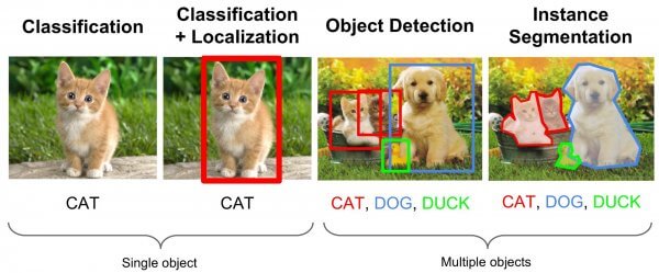
Image source: Review of Deep Learning Algorithms for Object Detection

How is SageMaker Different From RoboSat?

Although both support semantic segmentation on satellite imagery, they are very different platforms. Here are a few key differences:

• SageMaker supports a collection of tuned algorithms for everything from text classification to object detection and image segmentation. RoboSat is a tool tailored to semantic segmentation on satellite imagery and implements the U-Net neural network in the PyTorch framework.
• RoboSat is an end-to-end solution and provides data preparation tools out of the box. With it you can download aerial imagery from any Slippy Map compatible source, fully prepare your training dataset, train, and predict. SageMaker, on the other hand, provides a blank canvas with a number of examples and pre-built tools at your disposal.

We found that although automatic data preparation tools aren’t a part of the SageMaker environment, established tools like Label Maker pair nicely and complete the picture.

• Both toolsets can be run on GPU-enabled compute instances. One of the advantages of SageMaker is that, as part of the AWS ecosystem, provisioning and launching EC2 instances for your notebook hosting and training is super quick and straightforward. With RoboSat we set up a Jupyter Notebook in a Docker container that can be deployed to an instance of your choosing. SageMaker streamlines this process by asking the user to select the type of instance and automatically setting up the Jupyter server on the selected EC2. Training jobs can be launched from the notebook’s instance and will spin-up separate training instances.

Working with SageMaker

Our objective was to replicate, as closely as possible, the same workflow we used with RoboSat using the same (or very similar) data. We can break the machine learning process down into three steps.

1. Data preparation
2. Model Set up and Training
3. Prediction

In order to compare this process with RoboSat we maintained a few constants.

• The satellite imagery came from the same source, Mapbox.
• Our area of interest was the same area of Tanzania.
• The type of model is the same – image segmentation.

For the most part the pipeline looks similar. It is, however, worth noting a few key differences which make a direct 1-to-1 results comparison difficult (see our conclusion).

Data Preparation

Gathering and organizing data for Amazon’s newest image segmentation machine learning algorithm looks very similar to the process with RoboSat and is made simple using Label Maker. We can run through all of the data preparation on our local machine. No need to do this on a GPU-enabled instance.

We used the same area of interest as in our previous RoboSat experiment. After installing Label Maker we just needed a little configuration:

{
  "country": "united_republic_of_tanzania",
  "bounding_box": [38.9410400390625,-7.0545565715284955,39.70458984374999,-5.711646879515092],
  "zoom": 17,
  "classes": [
    { "name": "Buildings", "filter": ["has", "building"] , "buffer":3}
  ],
  "imagery": "http://a.tiles.mapbox.com/v4/mapbox.satellite/{z}/{x}/{y}.jpg?access_token=ACCESS_TOKEN",
  "background_ratio": 1,
  "ml_type": "segmentation"
}

Here, we’re telling Label Maker about our area of interest, the feature we’re interested in (buildings in this case), and the type of machine learning algorithm for which we want training data.

zoom represents the resolution of the satellite imagery and label data. In our previous RoboSat example we used a zoom of 19 but here, we’re using 17. The lesser zoom level will dramatically cut the size of the dataset and allow for quicker iteration and faster training.

With the configuration saved as config.json, we can continue through steps 1-4 on the Label Maker documentation.

$label-maker download will download the QA tiles from Mapbox

$label-maker labels will retile the OpenStreetMap label data and set the zoom level

$label-maker images will download the satellite imagery

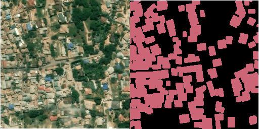
The above image contains the satellite imagery tile on the left and its corresponding label generated by the labels command on the right.

Once we have the satellite imagery and labels, we just need one quick tweak to use the semantic segmentation algorithm in SageMaker.

According to the docs SageMaker requires our labels (or annotations as they’re called here), formatted as single-channel 8-bit unsigned integers. Label Maker produces labels as RGB. Before uploading we converted each of our labels to a mode P PNG.

img = Image.open(label_path + '/' + file, 'r')
p_img = img.convert(mode="P")

For more details see the PIL docs.

With our training data downloaded locally, let’s upload it to an S3 bucket. SageMaker requires the dataset to be broken up into the required directory structure:

root
|-train/
|-train_annotation/
|-validation/
|-validation_annotation/

We split the imagery roughly 50/50 between the train/ and validation/ directories. The same can be done for train_annotation/ and validation_annotation/ (annotation in this context refers to our labels).

With our training data set, we can set up the model and train in SageMaker!

Training

To bootstrap our training setup, we used AWS’ image segmentation example notebook.

As we have already prepared our data locally and uploaded to S3, we can skip to the Training section of the notebook. We made just a couple small edits to the training configuration.

In defining the SageMaker estimator object we used a slightly smaller instance:

train_instance_type = 'ml.p2.xlarge',

• In our hyperparameter definitions we need to set to the num_classes param to match the number of classes present in the labeled training data. This will vary based on the input dataset and the value in the notebook reflects the Pascal VOC dataset.
• Define a label map. The AWS example does not require this step because the dataset they’re using (Pascal VOC) is mapped correctly. The labels we get from Label Maker are indexed slightly differently so we need to tell SageMaker how to interpret the class indexes.

We define the label mapping and write train_label_map and validation_label_map to a label_map directory in S3. For example:

import json
label_map = {
    "map": {
        "0": 0,
        "1": 134,
        "2": 98
    }
}
with open('train_label_map.json', 'w') as lm_fname:
    json.dump(label_map, lm_fname)

with open('validation_label_map.json', 'w') as lm_vfname:
    json.dump(label_map, lm_vfname)

Creating these two .json files and adding a label_map to our data channels will take care of our mapping. One thing to note is the validation_label_map.json. We need a map for training and a map for validation. In our case they should be the same values.

With those minor adjustments, we can execute all of the cells in the Training section. The last command, ss_model.fit(inputs=data_channels, logs=True) will start the instance and kick off training. Once training has started we should start to see metrics for each epoch (run through the training data).

Prediction

Again using the example notebook we can deploy our model to a public endpoint and use it to make inferences on images that were not part of the training data.

Conclusions

Our initial training run took about 4 hours on a P2.xlarge instance. The mIoU (mean Intersection over Union, our primary image segmentation evaluation metric) was a bit less than RoboSat’s initial output but there are several factors impacting these results.

• Perhaps most notably, we’re using a slightly different zoom level with SageMaker. In this post we’re using 17. In our RoboSat entry we used 19. That change presents a disparity in the size of the training dataset but allows us to train and iterate faster.
• We’re using a different model in a different framework. RoboSat uses a U-Net/PyTorch combination, SageMaker uses a custom Amazon Image Segmentation model directly in SageMaker.
• Our data preparation in this case is handled by Label Maker. Although both Label Maker and RoboSat are gathering imagery from Mapbox and generating labels, there could be variances in how labels are generated that impact the results.
• Our learning rate and number of epochs was the same between the two tests but there are a number of additional hyperparameters that could vary.

In the end, this isn’t meant as a benchmark or direct comparison between the models each pipeline produces. We are primarily interested in exploring the different workflows and illustrating two different but very related approaches to image segmentation on satellite imagery.