If you accept that we are living through the Tyranny of the Chunk, then you might be wondering how we got to this place. Who created the first chunks and what was their motivation? As we explore the history of different data formats we’ll see recurring patterns of thinking around how much information to consolidate in a single file. We’ll try to find the moment in time when the file abstraction broke and chunks fully became a concern for data consumers. And we’ll look to the future to think about ideas that might help free us of these concerns moving forward. So sit back and relax as we dive into a bit of story time.
A “history” of array formats
We’re going to use the word history loosely, or, perhaps more precisely: this is our account. What follows is our perception–it is based on maybe some facts and definitely on our own inferences. Primary sources are not necessarily easily available for everything we’re going to discuss, and we weren’t there for most of this timeline. We aren’t totally sure if we are right. In fact, we are probably wrong in parts. If you know better please tell us!
Early array usage
Arrays are among the oldest of data structures, given their use in mathematics, particularly for use in modeling matrices. Chunking arrays, therefore, also likely originated early in the history of computing. The term “out-of-core” dates back to at least 1962, and is a reference to data too large to fit into the main memory of a computer (as mainframe memory from that time used a technology called “magnetic core memory”) such that it necessitated some algorithmic chunking to facilitate processing.
The limitation of early computers led to this concept of chunking as a means of enabling any meaningful processing of array data too large to fit into memory–which back then could have been just a handful of kilobyes!
A little program called Landsat
Launched in 1972, Landsat 1 with its digital Multispectral Scanner (MSS) was the beginning of a massive volume of earth observation image data, all stored in raster format. Chunking at several different levels is a key feature of how Landsat MSS data was initially managed and made available. While a major component of the MSS chunking scheme was a product of hardware limitations, it’s notable that part of the data chunking was actually an organizational paradigm aimed at helping users find a subset of the data relevant to their needs!
The Computer Compatible Tapes (CCT) format developed for MSS data was designed specifically for the MSS, and was in many parts defined on certain key properties of the sensor and the nature of the produced data. Direct consumers had to have a deep understanding of the storage format, and by extension the sensor itself. Tooling was developed to abstract that concern from users, but then that tooling became specific to the MSS data, as the CCT format was not useful for other purposes. This problem was common to early data formats: they were sensor or otherwise hardware specific, and required either significant a priori knowledge to use or software tailored to each custom format.
See Appendix 1 for more details on the Landsat MSS CCT format.
A quick mention of FITS
Astronomy in the 1970s had a problem similar to Landsat’s. Except, instead of a common sensor platform like MSS, observatories had unique hardware and therefore unique formats. The lack of data and tooling interoperability was a major problem in the field, which led to development of a domain-specific interoperable data format in the late 1970s, and standardized in 1981 as the Flexible Image Transport System (FITS) format.
The original FITS specification did not leverage compression and was not exactly chunked, though it did enforce that data needed to be written in logical chunks of 2880 bytes within the larger physical blocks of the tape media. This requirement was intended to ensure data could be written and read in units compatible with and aligned to all the major computing platforms available at the time. In this way data chunking was leveraged within the format to handle the “out-of-core” problem, and did not provide any way to navigate within a stored array (it was expected that array data would be read sequentially from beginning to end).
FITS is worth calling out in this history not just because it was an early attempt at an interoperable file standard, but because it was designed as a self-describing data format. That is, FITS defined a mechanism for including arbitrary metadata within the file headers, allowing data producers to describe the following array data, including its shape, size, and other relevant properties necessary to parse the binary array data.
Early compressed formats
Landsat did not make use of compression: given the limited computing power and available compression methods of the time, any benefit of compression came at too great a cost. Tape was cheap.
Fax transmission formats
The first place where array compression really took hold was with digital fax machines, of all things. It turns out trying to push image data over slow phone lines meant compression was necessary for getting the whole thing to work–which sounds a lot like the case with cloud-native data today. As digital fax machines began to appear, each manufacturer ended up developing their own proprietary format, both because formats were tied to specific hardware implementations and to try to prevent consumers from switching to competitor’s machines.
It wasn’t until 1980 when the ITU-T T.4 (Group 3) fax standard was developed that a vendor-agnostic, interoperable specification was available. This appears to be the first formalized array format specification featuring the use of compression, specifically leveraging Run-Length Encoding (RLE) combined with Modified Huffman Coding to allow a high degree of compression for its 1-bit (black and white) pixel arrays.
Not only this, but ITU-T T.4 (Group 3) was chunked! Each scan line was compressed individually, as a separate chunk. Doing so allowed sending each line as it was scanned, rather than having to batch up and store larger amounts of data before transmission.
All this said, the ITU-T T.4 (Group 3) standard was not a file format, but a transmission format. It embodies the principles we’re concerned with in array storage, but isn’t strictly intended for it. So what was the first file format like this?
PCX: the PiCture eXchange format
It appears that the first widely-used format using compression to store array data was the PiCture eXchange (PCX) format from 1985. Similar to digital fax formats, this format used a specific RLE algorithm to compress image data along array rows. The data are row-interleaved depending on the number of “color planes” specified (typically 1, 3, 4 for grayscale, RGB, and RGBA imagery, respectively). In effect PCX ends up as a format chunked by rows in row-major order, which matches how it was intended to be used: as a format to store images for display on-screen, which requires reading the data line-by-line mapping to the screen’s scan lines.
PCX was among the first image formats to become a DOS imaging standard due to its widespread adoption at the time. It is notable because it was not connected to any specific sensor. It was a true software-focused image format, which allowed it to be generic enough to be generally useful.
The Tagged Image File Format
TIFF, the Tagged Image File Format, debuted publicly not long after PCX in 1986. Created by Aldus, the developer of the PageMaker software, TIFF was not just a software data format. Rather, TIFF was intended to be like ITU-T T.4 (Group 3) was for digital fax machines, but for scanners: a general specification that could unify all the manufacturer and device-specific file formats proliferating at the time. Because of this use case, TIFF had to be much more flexible in order to accommodate not just software authors, but hardware devices using different sensors, different amounts of memory, and various data interconnects, all with vastly different properties driving how they would be able to best store data.
Aldus looked at this problem and determined the solution needed to be transparent to users: the format needed to provide the flexibility required by data producers, but in a way that users wouldn’t have to care about. If they saw a TIFF file they should expect it to be openable by any application with TIFF support.
As a result, TIFF “steals” the idea of self-describing metadata from FITS. Of course, there’s seemingly no indication that TIFF developers were aware of FITS and intentionally took the idea from FITS, but TIFF is, chronologically, the next evolution of the idea FITS originated. This is the idea behind the format’s name: Tagged Image File Format. TIFF uses a different but equally-effective approach than FITS for storing image metadata, leveraging the concept of tags, which are like a set of pre-defined keys that map to binary values in the file metadata. Tags allow readers to have a constrained and consistent expectation of the possible metadata they will need to handle to be able to read any image, helping to ensure interoperability.
Unlike FITS, TIFF is a logically chunked format, using the term “segment” instead of “chunk”. All TIFF versions prior to 6.0, released in 1992, required images be segmented into strips. Unlike Landsat CCT strips, TIFF strips are groups of rows extending across the full width of an image. With version 6.0 of the specification, TIFF began supporting two-dimensional segments called tiles, with both a specified length and width.
TIFF is also notable for its compression support. From the first public version 3.0 it supported compression, borrowing the modified Huffman RLE scheme from ITU-T T.4 (Group 3). Successive releases of the spec added support for new compression algorithms, notably LZW in version 5.0 and JPEG in version 6.0. While the core specification has not been officially updated since 1992, support for additional compression codecs like DEFLATE and zstd has been added through supplements and widespread library adoption.
TIFF is still relevant today, perhaps entirely because of the seriously useful abstraction it provides for users: they get an interoperable file format, portable across systems and software applications, for which they don’t have to understand the inner workings. They don’t have to know exactly how the data is laid out on disk to be able to read or write to it. Sure, as we saw with the initial chunking discussion, some access patterns may or may not be efficient with a given tiling scheme. However, with data stored on a local disk, random access or extraneous byte reads aren’t generally that problematic, especially with modern hardware, so most users can safely ignore these concerns. In other words, the tyranny of chunks with local data still exists, but the costs are generally cheap enough to not be worth budgeting for.
Of course, now’s the time to queue jokes about TIFF as meaning “Thousands of Incompatible File Formats”. Sure, it’s true, the flexibility of TIFF means it has fewer guardrails to ensure data producers create files that will be widely compatible, breaking the abstraction. But within the geospatial domain, TIFF has been a fantastic foundational technology enabling the GeoTIFF, a profile built on top of the generic TIFF specification. GeoTIFF was first released in 1994. Consolidation around common tooling such as libtiff, or GDAL in geospatial circles, means that we’ve had 30+ years of consistency to converge upon common and interoperable usage patterns. Many people use TIFF because it just works across a wide range of tooling.
Despite the value of the file abstraction that we’re arguing for here, we also think it is super useful and informative to understand how TIFF works. The internet has some great resources for understanding this topic, though we’d like to point out a notebook from one of the authors that digs into a Cloud-Optimized GeoTIFF (COG) specifically as good starting point, as it aims to unpack both TIFF and the general concepts behind cloud-optimized data formats.
HDF and NetCDF
The late 1980s was a boom time for image formats, and we saw two major data forms arise: NetCDF and HDF, both of which were initially released publicly in 1988. Both aimed to be generic, self-describing array file formats, with even more flexibility than TIFF–real support for n-dimensional arrays was a crucial goal to support scientific uses where many data variables or additional array dimensions like elevation and time are common.
Today HDF5 has grown to be a highly featured data container, and is even useful for tabular data and other non-array formats. NetCDF has become somewhat of a format “profile”, with NetCDF actually adopting HDF5 as its backing data store format.
We could spend a lot of time on these formats, as they have been extremely influential with regard to how we’ve gotten to where we are today. They are both chunked and compressed, and heavily inform the design of Zarr. But the Cloud-Optimized Geospatial Formats Guide page for HDF/NetCDF does a better job than we could at explaining the formats in an easily digestible way, so we’ll just point to that.
Map tiles
The whole Web Map Service (WMS) era of the late 1990s and early 2000s is really the spiritual predecessor of our current cloud-native world. It is during this time that we see the desire to subset raster files over the network arise, motivated by the need to enable web users to load map data for arbitrary areas on demand.
The concept behind WMS originated in 1997, and it was quickly codified into an OGC API standard published in 1999. WMS queried data from backing files, subsetting and resampling the data for every request to match the viewport requested by the browser. This was not a scalable solution, however, because no two requests were likely the same and the required resampling operations could be computationally expensive.
Enter Google Maps. In 2005, Google ushered in a revolution with the unveiling of their Maps product. Maps showed the world what would become known as a “slippy map”, a super responsive web map UI that users could pan around in real-time, with quick performance. The key was pre-rendering the map images as XYZ tiles and serving them via a map tile service.
A particularly interesting and notable development for our discussion of chunks, the rise of map tilesВ is a clear point where we can see the concept of chunks transition from an internal, file layout concern to one exposed directly to data consumers! Map tiles are a definite precursor to what we see today in our cloud-native world, and seemingly served to normalize consumers needing to think about subsetting when consuming a larger dataset.
The idea of XYZ tiles is also interesting because we see them as something of an “external chunking scheme”. Instead of a file divided internally into chunks, we end up with many files representing a larger dataset. This is not so different conceptually from the Landsat path/row grid and how imagery was divided up into scenes, both to make data more accessible and to better accommodate technological limitations.
Cloud-native formats
Cloud-Optimized GeoTIFF (COG)
COG came about in 2014, not so much as a standard but as a grassroots-ish effort to make Landsat data more accessible (at this point in time we’d moved on from CCTs, to their modern equivalent: TAR files, literally Tape ARchives, wrapping a collection of GeoTIFF files). To be clear, a COG is just a GeoTIFF, but laid out in such a way that it can be read and subset efficiently over an object store interface like S3. COG also specifies that TIFF’s support for multiple arrays be used to store reduced resolution overviews, which enable more performant visualization.
COG is not so much a new file format; rather, it’s a convention for how to make reading GeoTIFFs more performant over a network. But with this convention comes a bit of a mindshift.
We start to see the community considering how to make data accessible without anything more than object storage: can we just put a file in S3 and let users access it directly, no servers required? It’s kinda the idea from map tile services, but more generic: can we access data performantly over the network not just for visualization, but for analysis as well?
It is here that we begin to lose the grip on the file abstraction that TIFF et al. so kindly brought to us, helping us to not have to worry quite so much about how we are reading and writing data. With COG we start to have to consider our tile sizes and overview levels. As producers we have to think much harder about how the data is going to be used by consumers, and to make sure it is structured to accommodate their needs. And, as consumers, we begin to have a vague awareness of how particular COGs were produced and if they will performantly support the required access patterns.
Zarr
Zarr began in 2015 as an experiment to find a more performant way to store array data in genomics. It has since expanded its reach across the sciences and into geospatial. While not originally a format targeting cloud use, it has also proven to be well suited to the cloud-native paradigm, providing highly performant data access to cloud-hosted n-dimensional arrays. Zarr, at least conceptually, builds heavily off earlier data formats like HDF. Zarr is also not just an array format, it is a group construct as well.
Zarr v3 supports two storage paradigms: “normal” (for lack of a better term), and “sharded”. Normal Zarr is kinda like combining TIFF and XYZ tiles: data is split into n-dimensional chunks, and each chunk is stored in an individual file. Sharded Zarr is also chunked, but the chunks are consolidated into larger blocks–essentially we get chunks of chunks. Each of these “chunks of chunks” are then written as files, with an additional index to allow looking up where in the file a given chunk resides. Shards are a lot like a TIFF file without additional metadata and with a different index format.
Because of the n-dimensional nature of Zarr data, chunking can be a much more complicated topic than with formats like TIFF, where chunks are limited to two dimensions. Zarr also doesn’t have the same conventions around how to store data to accommodate performant visualization. Both of these factors make chunking even more of a concern when using Zarr data.
Cyclical themes
This section is a bit of an aside, but it is interesting to consider the themes we see as we look through this brief history. The main ones tend to be about consolidation vs separation: do we put these things together, or do we split them apart?
The file is too big!
We see this argument arise as data size increases faster than storage availability. Some newer way to organize the data comes along, or a new format that splits the data apart into multiple files gets popular. Until the pendulum swings back the other way, of course, and the argument becomes “there are too many files!” We see this right now with Zarr and the need for sharding to reduce the numbers of chunk objects, make stores more manageable, and allow read coalescing across smaller chunks.
The format should capture the data hierarchy/relations!
This one might just be a spin on the first point, but it goes like this: should we group data sets together into a single file, or do we separate them out into multiple files? Should overviews be in the same file, a la COG? Or should they be in a sidecar file? Should we bundle related datasets together, in an HDF/NetCDF/Zarr/TAR? Or should we keep them separate so they can be consumed independently, such as was done for Landsat with the advent of COG?
Zarr seems to want to consume the world but still allow independent consumption. Except how can an array format contain the relationships between all data? If Zarr cannot adequately model all data with its hierarchy, should we put any grouped data together?
All the metadata should be included!
This is a hot topic right now around the intersection of Zarr and STAC. Does STAC-like metadata belong inside the data format? Does metadata even need to be stored externally?
TIFF vs Zarr actually shows a perhaps unexpected version of this concern: TIFF, necessarily, has to contain an index conveying where tiles are within the file, where Zarr does not have to index its chunks at all–it can offload that responsibility to the storage layer. That said, tracking where the chunks are is important, it is metadata, it’s just not in the Zarr.
Virtual Zarr stores introduce an interesting wrinkle by essentially capturing all the metadata from a multitude of files and (in the kerchunk case) storing all that metadata in a central file. That central file tells readers where to get the bytes of data from (like TIFF metadata) but it is stored separate from the data files themselves.
Another version of this theme could be the current debates around consolidated metadata within a Zarr store: should we or should we not put metadata for the whole hierarchy into a single file? Argument for: it gives you everything with one request. Argument against: it won’t scale.
COGs don’t allow arbitrary metadata to be included within them. This is why there is an entirely separate mechanism for tracking and managing metadata – STAC. This means that COGs are not entirely self-describing; you need the STAC metadata to know what time a satellite image represents. It also makes it easier to update the metadata without having to modify the datafiles at all.
Isn’t this just a variation on “the file is too big?” Maybe these are all just different expressions of the same concern?
So, where are we now?
As we look back through this history it seems like we gained a valuable abstraction when we got self-describing data formats. Maybe it’s a little bit leaky, but for most users it was good enough. Along the way though, the bucket broke, and now the water is pouring out. We’ve lost the abstraction in some pretty significant ways. And, as we see larger and larger datasets move into the cloud, and in particular adopting Zarr and pushing more cloud native workflows on more users (for all the benefits they bring!), it seems like the conversation–or, maybe, confusion–around chunks just gets more intense.
The way we are using chunks today is perhaps different than how they were originally conceived to be used. We see this manifest in Zarr stores as chunks sized at 100MB+ because they’ve become an atomic unit of access. These chunks cannot be subdivided, but they can also not be consolidated–this latter constraint is novel.
Even in other formats like COG, where reads can be coalesced, they typically cannot be coalesced perfectly. And often we need to access data across many COGs. Our chunks begin to fail, because they do not model how data may be composed together across arrays. And we find the additional latency simply exacerbates the costs.
So maybe we should ask ourselves, in trying to fight to find the optimal chunking solution, are we even asking the right question? Might chunks no longer be the right way to model our access problems anymore?
Maybe chunks are still good, maybe we just need another abstraction to help us use them better, to better mitigate the impact of unaligned chunks? Or has the scale of our data changed the optimal solution, and we need a completely new paradigm?
Can we tame the tyranny in some way? Or do we need a usurper?
Where might we go from here?
We see two possibilities, though there certainly could be many others.
Reconsider what it means to be cloud native
Can we get back to a world where access pattern misalignment is again not expensive enough to care about, except maybe at the largest of scales? 99% of users could go back to not worrying about this problem, and data producers could default to a single, hopefully-optimized approach to chunking.
This idea sounds great, but how do we do it? We’ll admit, the how here is not exactly obvious. That said, we know that chunking worked pretty well with local data. Can we mimic how local data access was performant? By this we do not just mean implementing data-proximate compute. That approach certainly helps with latency problems but you are still accessing data over HTTP using linear-only subsetting. What if instead we move chunk resolution and consolidation even closer to the data, putting it behind the HTTP interface? Doing so would make it possible for users to make a single request to retrieve data across chunks and objects.
Solutions like OPeNDAP aim to do this by offering an array-native API, but end up being computationally intensive, require management, and are ultimately not cloud native. Is there a solution like this that could be as performant as S3, but more array-native? Cloud native has come to mean “uses object storage.” Maybe we need to reconsider what cloud native means: perhaps we’ve gotten stuck at local maximum, and we can do better than the S3 API?
Reconsider data
Maybe a response to chunking being so ineffective is to change the way we look at data entirely!
Let’s lean in to information theory, and let’s question what our data actually are. Much of an array dataset might just be noise polluting the relevant signal. We see a tremendous amount of spatial and temporal correlation within our data, perhaps we should consider compression techniques that can remove that noise without reducing the signal and give us smaller representations of the data on which to operate.
AI is already taking us in this direction. Vector embeddings, one of the core ways to represent semantic meaning to LLMs, is in essence a form of lossy compression which reduces dimensionality while preserving semantic relationships. PCA is an older version of similar concepts. Many newer techniques for reducing dimensionality exist: could we find a way to leverage tools like these to reduce our data while retaining utility?
Again, the how is not obvious here, but the research and possibilities are exciting! A breakthrough in this area could be game changing.
Conclusion
We’ve surveyed quite a lot of the chunking landscape between the Tyranny of the Chunk in part one and the origin of chunking here in part two. From all of this, we think it is clear: chunking is complicated! Processing data at all is complicated! That any of this technology stuff works at all–let alone so well that it enables the innovation it does–is pretty incredible!
As we said in part one, chunking is complex because it embodies the intersection of three orthogonal issues:
- The data use cases, i.e. how do people and software want to use the data.
- The performance characteristics of the data’s retrieval, specifically with regard to storage and data transfer.
- The role of budget: how to prioritize processing costs versus storage and/or transfer costs.
This complexity of chunking is inescapable as long as we have large multidimensional datasets that must be linearized for storage, transmission, and/or processing. Multidimensional computing and storage architectures might eventually help, but it is unlikely within any reasonable timeline that we will find a means to remove the need to linearize entirely. Until then we are stuck with the tyranny of the chunk.
That said, it seems much more feasible that we find ways to mitigate the effects of chunking’s tyranny than to be able to remove the need for it entirely. We presented two possible but fuzzy paths to consider towards this goal:
- Reconsider what it means to be cloud native – can we mitigate chunking impact by building better data interfaces?
- Reconsider data – can we mitigate chunking impact by reducing the size of our datasets through better compression and deduplication techniques?
Both these options need much more thought and development before they might become viable for our community. And they are certainly not the only options that we should be considering.
So, we want to open this conversation up: if you have thoughts or ideas about these options or others, please, let us know! Or, better yet, write about them somewhere online and send us a link! Especially if you disagree with us about any of this.
Appendix 1: Additional details of the Landsat MSS CCT Format
Unpacking the Landsat MSS CCT data format requires understanding a bit about the MSS sensor. The MSS was a four-band whiskbroom sensor, which imaged across the orbital track six scan lines in each band at a time using an oscillating mirror to capture a 185km wide swath. As the satellite moved forward along the orbital track the scan line groups would progress forward. The data produced by this sensor was recorded onto two onboard tapes, the wideband video tape recorders, each of which could hold about 3.75 gigabytes of data to buffer data between ground station overpasses.
Downlinked data would be recorded at ground stations on high-density tapes in the same continuous raw sensor format. The raw data would then be processed into a “standardized” L0 data format stored across four CCTs. To constrain the amount of data being processed at any given time, and to facilitate more effective data organization, the raw swath data was split into sections of 2,340 scan lines forming an image scene approximately 185km long by 170km wide. These tiles were referenced by their path and row coordinates, forming the Landsat tile grid we still use today, and serving as an effective spatial chunking unit.
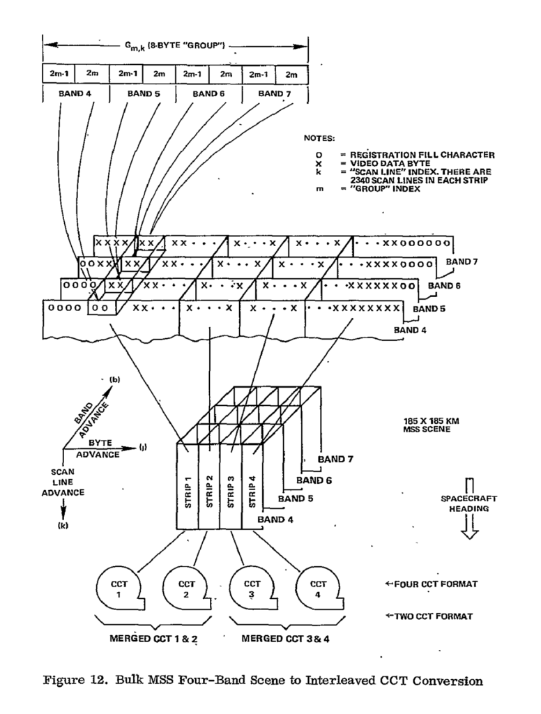
Within a CCT scene, the data were chunked into two groupings. First, the scene scan lines were divided up into four strips–this was necessary because the CCTs were not large enough to contain the entire scene, so four CCTs were required, each containing one image strip. Perhaps contrary to expectations, these strips were oriented along the length of the image, and split scan lines across each CCT. Within each strip the values for each band were interleaved, with two consecutive values per band (6 or 7 bit integer values padded to 8 bits) forming an 8-byte long “group”. This format might appear a bit strange from a modern perspective; it seems perhaps easiest to conceive of this as the data were chunked into 2 pixel wide by 1 pixel long by 4 band tall chunks, then stored in row-major order within each strip.
Landsat CCT is a particularly interesting format for us because it is both an early and well-documented format that captures the ideas that array data can be split to accommodate storage, processing, and organization needs. Note that the chunking scheme does not need to be overly concerned about specific access patterns, as without compression it is technically possible to randomly seek to any given group or pixel by calculating the offset within the larger strip data structure (not that doing so was particularly fast given the tape storage medium). Landsat CCT might not be the first array storage format to use these principles, but it is perhaps the largest scale use-case of the time period.
For a more in-depth review of the CCT format, see the following references: