Recently, the E84 R&D team has been experimenting with machine learning pipelines and identifying potential use cases. There are a lot of new and exciting tools out there and we’re interested in exploring what’s available, particularly tools related to satellite and aerial imagery (one of our specialties). Mapbox‘s RoboSat was released earlier this year and is described as “an end-to-end pipeline written in Python 3 for feature extraction from aerial and satellite imagery.” We’re excited about the possibilities and would like to share what we’ve learned!
Our introduction to RoboSat was this excellent blog post from Daniel J. H. on the Mapbox team. It’s a fantastic walkthrough of the entire RoboSat process, describing how a user can select an area of interest and use it to train a model that accurately identifies features in satellite imagery.
Why RoboSat?
We chose RoboSat because it is a specialized open source toolset that allows us to work with satellite and aerial imagery out of the box. The data preparation is largely handled by the pipeline so we’re able to get to the good stuff quicker.
Although RoboSat can be extended to support just about any aerial imagery and labeling data you might need, we opted to use natively-supported providers. We used Mapbox for our aerial imagery and OpenStreetMap for labeled training data.
What does RoboSat do, exactly?
At its core, RoboSat provides easy-to-use abstractions for all phases of the machine learning process. From the RoboSat README:
- Data Preparation: Creating a dataset for training feature extraction models
- Training and Modeling: Segmentation models for feature extraction in images
- Post-Processing: Turning Segmentation results into cleaned and simple geometries
Essentially, this means that we can take raw data from a source like OpenStreetMap and combine it with satellite or aerial imagery from a source like Mapbox or OpenAerialMap to train a machine learning model that can predict one of a number of supported features. In our case we’ll be looking at buildings as a starting point but anything for which OpenStreetMap has a label, you can detect using RoboSat by writing a small custom handler.
Here’s an example:
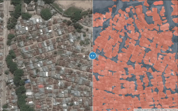
In the above image we can see the original satellite imagery on the left and the model’s prediction of where the buildings are in that imagery overlaid on the right.
Give it a Try!
To help share our progress internally with the E84 team and make life a little easier for those getting started with machine learning, we’ve created a Jupyter Notebook with all of the steps outlined in the original blog post. Each step can be executed immediately without additional prep outside of the notebook. To get started, take a look at the README for set up instructions. We are training a machine learning model on a large dataset so, although all of the steps can technically run on a CPU, we would strongly advise running the notebook (or at least the training) on a GPU-enabled machine. We used AWS’ P2.xlarge instances. Take a look at the README for details.
Our Results
During the training process, the function will output “checkpoints” at a set interval. Each checkpoint, generated at the end of each “epoch” reflects one entire training run through the training dataset. The number of epochs (runs through the training dataset) is a tunable parameter and the metrics given at each checkpoint can also be extended. For our experiments we were primarily concerned with the Intersection over Union metric.
The initial training of our model produced pretty decent results. In our research we found that the mIoU, or mean Intersection over Union, was ultimately the most meaningful metric for determining the quality of the model. Essentially the Intersection over Union is the overlap of the “ground-truth” bounding box and the predicted bounding box. Our pre-labeled training data (OpenStreetMap) was already labeled with these bounding boxes so the object here is to compare these bounding boxes with those predicted by our trained model. The closer the two, the better the IoU and the better the model’s prediction. Here’s a good explanation of mIoU.
According to this article, “An Intersection over Union score > 0.5 is normally considered a “good” prediction.” Our original model was in the “good” range with an IoU of about 0.56 but it could be better. There are a lot of possibilities for tweaking a models performance. We could:
- Provide a larger dataset. If we are creating our own training data, we could add more labeled data.
- Adjust a few of the tunable parameters in the RoboSat config such as the learning rate, batch size, and number of epochs. This is referred to as “hyperparameter tuning”.
- Add negative samples to the dataset.
Let’s talk about that third option as, in our experience, it is the most promising.
Improving the Model with Hard-Negative Mining
Looking at our predictions, one problem that is immediately obvious is that we have a lot of false positives. We’re seeing labels appear, claiming that there is a building where there is clearly no building. This is due largely to an imbalance in our dataset. We’ve given the model only images with buildings. Those images also have background but there are going to be far more building pixels than background pixels on the whole so the model is not going to have enough information to confidently say what is not a building. One solution to this problem is to provide the model with images that do not contain any buildings.
Validating that an image does not contain a building is a manual process no matter how you cut it. RoboSat provides tools to assist but we found the easiest (though not necessarily best) way was to write a small feature handler for the pipeline. It is included in the notebook and allows us to download all tiles that do not contain a building. Once we have a few we can manually verify that “yup! This tile does not have a building in it!” and add it along with an associated blank label to our dataset.
Now that the model has a collection of “negative” images as well as images with buildings, our predictions should contain fewer false positives.
Conclusions and Lessons Learned
This was an excellent introduction to RoboSat for the E84 R&D team. We were able to produce a good segmentation model relatively quickly and get a feel for the process of tuning it. Here are a few of our key takeaways:
- The resolution of the satellite or aerial imagery is important. We opted to use Mapbox imagery as opposed to OpenAerialMap for better coverage of our area of interest. An interesting experiment would be to directly compare the model trained on Mapbox data with a model trained on OpenAerialMap data at a higher resolution.
- Hard-negative mining is a very time-consuming and manual process. If our original dataset contains 400,000 tiles, it would be quite a large undertaking to provide enough negative tiles to make a difference in the prediction.
- One step that’s not included in some of the walkthroughs that we’ve seen is the matching process before training. RoboSat’s
trainfunction requires the same number of labels as satellite images. If you download your satellite imagery from a source like Mapbox or OpenAerialMap using thers downloadhelper, it’s possible that it won’t have every tile you’re interested in. As we generate our labels separately, we may have labels for which no image is available. We’ve written and included a small Python snippet in the Jupyter Notebook that handles this discrepancy before training.