It is a truth universally acknowledged in cloud native geospatial that data formats must be chunked. There are many best practices guides and rules of thumb on chunking–this post is not one. This is our attempt at trying to understand chunking more deeply: where we are today, how we got here, what we’ve gained and lost along the way, and where we might want to consider going from here.

This is the first post in a two part series. In the second part, we tell an origin story of chunking and explore what that might tell us about the road ahead – check it out here. 

Why we are writing this

We started writing this post thinking about chunking arrays and how to choose the optimal on-disk layout. People refer to chunk patterns as if they were a dark art of some kind, except concrete technological constraints underlie optimal chunking schemes. We thought there must be a right answer, but, as we started picking them apart, we realized this subject quickly gets quite complex and potentially confusing.

As we thought about this more, we had a difficult time justifying why a scientist or other data consumer trying to save some data should need to think so much about how the file itself is structured. Isn’t the point of standardized file formats that you don’t have to think about the actual bytes and how they are arranged on disk when you are reading or writing data? So how did we get to this place? Where did we lose that abstraction?

Why chunking matters

Chunking decisions happen at the intersection of three orthogonal issues:

• The data use cases, i.e. how do people and software want to use the data.
• The performance characteristics of the data’s retrieval, specifically with regard to storage and data transfer.
• The role of budget: how to prioritize processing costs versus storage and/or transfer costs.

Before we get too far though, let’s start by building up a shared understanding of what chunking is exactly and how it has come to embody these different issues. Be aware, we are going to get deep into this, and we might dive off onto a number of what seem like tangents, but please bear with us, we think it is (hopefully 😅) worth it.

Note that this concept of “chunking” applies to many data types, and some of what we say here will apply universally, but our focus is specifically on raster/array data.

Chunking fundamentals

Computer storage systems are intrinsically one dimensional. In RAM, on an SSD, on a network file system: in each case data is stored as a linear sequence of bytes. Data transfer is also one-dimensional. Think of data being read off disk or sent over the network – both are again a linear stream of bytes.

Raster arrays, however, are inherently multidimensional. Consider an array representing a satellite image: it minimally has a width and a height, making it two dimensional. Add multiple bands to the array and it becomes three dimensional. Climate data can often take this further, adding a temporal dimension, a third spatial dimension to capture elevation, and many different data variables pushing our dimensionality further and further away from its necessarily one-dimensional representation in storage.

This discrepancy is more than just a curiosity. It creates an impedance mismatch, one represented by this fundamental question: how do you flatten multi-dimensional data for storage in a one-dimensional medium?

Equally important is the corollary: how can you transform a linear sequence of bytes into a multi-dimensional array and perform multidimensional operations upon it?

The answer to these questions is chunking. But what exactly is chunking? Let’s dive into some examples of how we can lay out arrays in storage to understand this better.

(For those that want to dig deeper, the concept here is generalizable as one of “linearization”. This is an interesting concept in computer science that applies to array data structures like we’re discussing here, and also to the analysis of operations in concurrent systems and algorithms.)

Array storage layouts

Row-major layout

A traditional approach to array storage is row-major ordering, also known as “C-order” (after the C programming language). With row-major ordering, each complete row gets stored sequentially before moving to the next row.

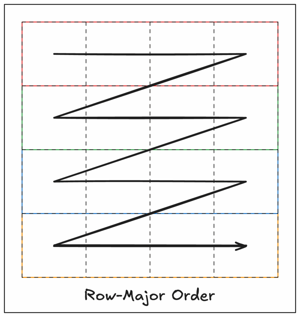
For example, given a two-dimensional array of size 4×3 like:

[[0,  1,  2,  3], 
 [4,  5,  6,  7], 
 [8,  9, 10, 11]]

C-order would represent this array in one dimension like you read text on a page, left-to-right and top-to-bottom, like:

0 1 2 3 4 5 6 7 8 9 10 11

If we know the size of the array (from external metadata) then we can read this one-dimensional representation of the data and convert it back into its two-dimensional form. For this example, we know that our array is 4×3, so we can calculate our row and column coordinates using:

row = floor(index / 4)
col = index % 4

Row-major ordering works exceptionally well if you need to read entire rows. But what if you want to read a single column, top to bottom? You’d have to either: 1) jump around in storage, reading every nth element, or, 2) read the entire array into memory and throw away all the parts you don’t want. Neither of these is ideal…

Column-major layout

Enter the column-major layout! Also known as “Fortran-order” (because, perhaps obviously, this models how Fortran stores arrays in memory), column-major order is essentially the opposite of row-major and stores complete columns sequentially.

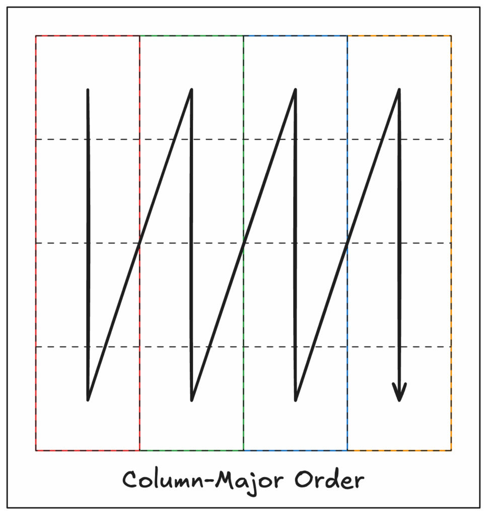
The same example 4×3 array from above would be stored as:

0 4 8 1 5 9 2 6 10 3 7 11

This strategy optimizes for column access, but by doing so makes row access inefficient! This is in effect the inverse of row-major ordering. Both approaches suffer from the same fundamental problem: they optimize for one access pattern at the expense of others.

Chunked layouts: the best of both?

Chunked layouts break arrays into smaller, multidimensional blocks called chunks (or tiles, strips, segments, blocks, etc. depending on the domain). Instead of storing the entire array in row-major or column-major order, the array is divided into rectangular (or hypercubic for higher dimensions) regions.

Let’s consider our 4×3 array, but this time let’s see what it would look like split into 2×2 chunks:

Chunk 0: 0 1 4 5
Chunk 1: 2 3 6 7 
Chunk 2: 8 9
Chunk 3: 10 11

On disk (in chunk-row-major order): 0 1 4 5 2 3 6 7 8 9 10 11

Now, accessing any rectangular region requires reading fewer, larger contiguous blocks rather than many individual elements. We have compromised between the row- and column-major access patterns: if we want to read a row we have to read two complete chunks, or twice as much data as a single row in row-major order. But if we want to read a column it is the same: we read two chunks, instead of the entire array, which is half as much data as row-major order!

In effect we have found the midpoint between the two extremes of wanting a row vs a column, neither of which, as it happens, is a commonly accessed shape (for the majority of raster datasets and use cases, that is). Instead, users generally are more likely to want data within roughly rectangular regions, so we optimize for that case, and in doing so we end up with the not too terrible compromise for row vs column access.

Note that of the above three layouts, it turns out all three are chunked. The row- and column-major are just two different edge cases of chunk shape and size. In the row-major case, our chunks are 4×1, and in the column-major case our chunks are 1×3.

So are chunked layouts the best of both the row-major and column-major cases? No, of course not, because if all three are chunked layouts then this question is nonsense! Instead, what we really need to be talking about are chunk shape, size, and how these factors impact efficient data access. We also might realize chunks split our linearization concern and push it in two separate directions. We find we still need to linearize:

• The data within our chunks: do we use row-major order, column-major order, or some other order for this?
• The chunks themselves: after chunking we still have an array to store! It is an array with smaller dimensions–2×2 instead of 4×3 in our example–but it is still an array, where each cell itself is an array (chunk). Again, do we store our chunk array in row-major order, column-major, or something else? …Do we chunk our chunks?

Generalizing these points a step further:

• Chunking is potentially a recursive process, which we could do as many times as makes sense (but how many times makes sense?).
• Chunks of chunks are inherently a different concept than a chunk, because chunks are composed of values, where chunks of chunks are composed of, well, chunks.
• Given our list of ordering options “row-major order, column-major, or something else”, we probably ought to think a bit more about the “something else”…

Space-filling curves: a possible “something else”

To linearize our data/chunks, we need to have an algorithmic way to establish a one-dimensional order from multidimensional coordinates when writing data, and to reverse the one-dimensional order into multidimensional coordinates when reading. Row-major order is a super simple algorithm for this transformation: go across a row until you get to its end, then start at the beginning of the next row and do that again. Column-major is likewise as simple.

But what other options do we have here? We need some way that ensures we visit all coordinates in the array (turns out in mathematical terms what we want is a “self-avoiding walk”), but also conveys meaningful enough advantages over row- or column-major ordering to warrant any additional complexity.

It turns out there are other linearization algorithms that are worth considering. These come from mathematical analysis, specifically as the concept of “space-filling curves” (here’s a great video). Some of these get pretty wild (see the Dragon curve) and aren’t super useful for our purposes, but it turns out two are really interesting to us here: the Z-order, or Morton, curve and the Hilbert curve.

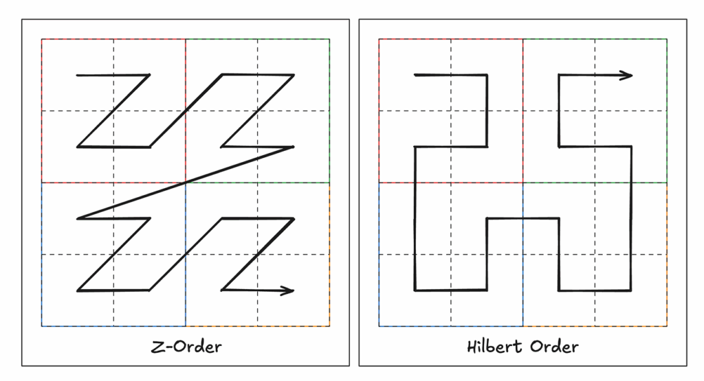
Both the Z-order and Hilbert curves give us a way to linearize a multidimensional array into a single dimension while preserving a greater degree of spatial locality.

Should we use these space-filling curves to order the data within our chunks, or our chunks themselves? Well, maybe.

Both work well when considering two-dimensional access patterns, because each maps well to the “tile-oriented” nature typical of 2D raster access. But, especially as dimensionality increases and access patterns become more variable, it becomes easier to find exceptions that don’t map exactly to either curve. Moreover, using these space-filling curves for ordering means that we cannot simply append new data to a file: adding chunks/pixels requires considering if the new data necessitates reordering/rewriting the entire file to ensure spatial continuity is maintained.

For a more hands-on space-filling curve resource, and to see how dramatically ordering can change based on grid size, check out this web tool for generating Hilbert-like curve approximation for arbitrary grid sizes.

Is there another “something else”?

Yes, certainly! It’s possible to try to throw out linearization entirely, at least at higher levels like chunks, where we can question if we have to treat this as a linearization problem at all. And this isn’t just a thought experiment: Zarr does this in practice! Zarr chunks in an object store are often stored as separate objects, which can be written and read in parallel–thus can be stored and accessed in a non-linear fashion.

Of course it is important to note that linearization still does apply here, just at a different layer. Using a file system to track which bytes on disk correspond to those for a given chunk means the file system is responsible for the linearization of chunks within the larger disk. After all, a disk is “just” a big long string of bytes split into blocks. And object storage is similar, in that it maps object keys–file names–into their constituent blocks of bytes stored, ultimately, on backing disks (though to be fair, even this mapping may not be particularly linear depending on implementation, as blocks can be sharded across multiple backing drives and accessed with some level of parallelization).

Wait a minute! Now we’re talking about file systems? And splitting chunks up into…blocks? Remember we started this whole section with the statement “computer storage systems are intrinsically one dimensional”. It turns out this idea of “chunking” is a more general concept in computing, and if we dive deeper into the meaning of “storage” we’re going to see this concept pop up in a number of different but related ways. 

How chunks map to storage

All storage mediums have an optimal access granularity, or a specific size of data read or written in a single operation. Exactly what in the system is the limiting factor for read/write performance can be hard to reason about. We’ve compiled a list of potential things to consider in Appendix 1, for those that want to dig in more deeply. 

Thankfully, for our main purpose of considering multidimensional array chunking for storage and access, file system block size is often the most influential factor to consider when reading and/or writing array data from/to a local disk. Here, assuming uncompressed data (a big assumption), sizing your chunks as closely as possible to a multiple of the block size is likely the most efficient strategy (and smaller is also probably better, depending on how you resolve the chunk positions: if you use an external index then the lookup overhead of small chunks might be too high, except here with uncompressed data we should be able to calculate the byte slice to retrieve any specific chunk, or even cell).

That said, the other granularies are important to recognize when considering how data is stored and accessed for things like NumPy arrays materialized into RAM, and how you ultimately are needing to process the data values. Most processing workflows will likely require several levels of chunking, and even rechunking to get data values colocated and aligned in memory in non-obvious ways to optimize for the different unit boundaries enforced by the different levels of data access within the system.

Chunks over the network

Of course, in our cloud-native world, when we are talking about chunk size we’re often not considering the intricacies of the local machine doing computation, but rather how we store and access data in cloud object stores like S3. Instead of thinking about how to move large amounts of data very short distances within a computer over reliable, high speed interconnects, we now have to consider that same data moving over significantly longer distances, across relatively slow and inherently unreliable network connections. Even colocating compute with object storage, such as EC2 instances in the same region as an S3 bucket, the difference in request latency and effective data throughput compared to local storage can be significant.

Consider: object storage uses HTTP as its interface. Generally speaking, HTTP runs over TCP. TCP is a “reliable” transport protocol in that it guarantees data will make it to the other end, but not how fast or efficiently that will happen. TCP can make it difficult to saturate a link, and often necessitates a higher layer coordinating multiple connections to get close. How all of this works and the underlying concerns, like storage access granularity, quickly get complex as one digs in deeper.

We’ve bullet-pointed some thoughts that come up as we think about the networking problem in Appendix 2, for those that want to consider this more.

For many workloads, strategies for making data access efficient locally, such as chunk alignment to disk blocks or how to optimize array data laid out in RAM for fast CPU access, quickly become irrelevant to performance relative to trying to optimize data access over the network. Unfortunately, how to optimize data access over the network quickly becomes specific to the network conditions (latency, bandwidth, reliability) between the data source and client, what access patterns are required by the client’s workload, and the shape of the data itself. Therefore a “one size fits all” approach to these problems is often particularly hard to come by.

Chunks and compression

One consistency between locally and remotely stored data is the effect of compression, and this is important over the network too. Compression is a critical technology when it comes to reducing the disk space required to store and bandwidth required to transfer both large and small arrays.

And it turns out that compression is particularly important to consider in any discussion of chunking. To understand this, let’s turn back to our example 4×3 array.

When we compress array data, what we are specifically compressing are the data values in our array. This might be a ridiculously obvious statement, but it highlights a key point after our discussion of chunks of chunks and whatnot: we need some set of our array data values to compress together.

Now, naively, this could just be the complete array. In the case of our 4×3 array that might make a lot of sense (if we deem it reasonable to compress at all, of course). Let’s see what we get if we do that!

>>> import zlib
>>> import struct

## we'll assume linearization has already happened, here in row-major order
>>> array = [0, 1, 2, 3, 4, 5, 6, 7, 8, 9, 10, 11]

## we use struct to pack our array into INT32 values
>>> packed = struct.pack('I'*12, *array)
>>> len(packed)
48

>>> print(packed)
b'\x00\x00\x00\x00\x01\x00\x00\x00\x02\x00\x00\x00\x03\x00\x00\x00\x04\x00\x00\x00\x05\x00\x00\x00\x06\x00\x00\x00\x07\x00\x00\x00\x08\x00\x00\x00\t\x00\x00\x00\n\x00\x00\x00\x0b\x00\x00\x00'

## compress with no header
>>> compressed = zlib.compress(packed, wbits=-15)
>>> len(compressed)
27

>>> print(compressed)
b'\r\xc3\x87\r\x00\x00\x03\xa0\xba\xd7\xff\xff\n\tIR\xac6\xbb\xc3\xe9r{\xbc>?'

Notice that our binary data (packed) is exactly what we might expect: we get four bytes in our binary string per value (4 * 12 = 48). This also means we could slice it however we need to get the value for any given cell (using its linear index, of course).

Once we compress, however, we no longer have a way to index into any given cell. How many bytes in the compressed byte string is a given cell? In fact, that question makes no sense: the compressed string is a single unit, we can’t make sense of a part of it without having the whole (with certain compression algorithms this statement is not strictly true, but in general the point holds).

Understanding this point we realize: if we compress the entire array we must have all of the compressed data to read any portion of the array. In other words, any subsetting must be done prior to compression.

Another key point about compression: the more data we compress together, the greater the compression effectiveness (though the degree to which this is true depends on the data, the compression algorithm, and how they interact together). Compressing a short length of data can actually increase its size, which we can see with our example case if we use a shorter data type (one byte):

>>> len(zlib.compress(struct.pack('B'*12, *array)))
20  # compared to the uncompressed length of 12

And getting better compression is important! Any gains in compression efficiency save money on storage, and reduce the environmental costs of storing large data sets. We can also save money when sending data over the wire because cloud egress costs can be extremely high. Not to mention time: more bytes over the wire mean we have to wait longer for all of the data to get to the other end. With modern CPUs and compression algorithms, often the processing time required to compress/decompress the data is significantly less than the time saved by sending fewer bytes over the wire.

These two points about compression are a bit at odds. We want small subsets of our array to allow more granular access (small chunks), but we also want to compress together as much data as possible to get more effective compression (big chunks). We need to balance these two conflicting needs. That balance point depends on the structure of the data itself and how it is being stored – in particular, the compression algorithm. Finding that balance point will give us a strong indication of the appropriate chunksize.

This is an important realization: chunks are our unit of compression, as well as our unit of data access.

Compression effectiveness generally grows logarithmically with data length, so after a certain point compression gains are significantly limited. Thus, smaller chunks (1-10 MB of data uncompressed) often compress quite well, and larger chunks can actually end up being less performant for general access patterns because they increase the likelihood that data sent over the wire to the client wasn’t actually wanted.

Of course, if we are storing the data in an object store and we have to make a separate HTTP request for every chunk we want, that won’t be efficient either. We’ll have to wait a whole round trip to get every chunk, and if we want a lot of chunks–because they are small–then we could be waiting a long time. Parallelism can help quite a lot here, but there’s only so many requests we can make in parallel, and we still have the problem of having to wait the time to first byte within each of those requests to even be streaming any data. Could we instead/also mitigate this problem by somehow making fewer requests?

Read coalescing

If we can use read coalescing, yes! Can we use read coalescing? Well, maybe.

Let’s take a look at some examples. We’ll use our chunked example array. Remember it looked like this:

Chunk 0: 0 1 4 5
Chunk 1: 2 3 6 7 
Chunk 2: 8 9
Chunk 3: 10 11

On disk (in chunk-row-major order): 0 1 4 5 2 3 6 7 8 9 10 11

We can create a chunk index into our on-disk data by tracking the starting byte index and length of each chunk:

Chunk 0 start, length: 0, 4
Chunk 1 start, length: 4, 4
Chunk 2 start, length: 8, 2
Chunk 3 start, length: 10, 2

In this case, if we want chunk 0 we can make an HTTP GET request to our object store for the object with this array data, and set the Range header on the request to bytes 0-3. And if we want chunk 1 we’d use the range 4-7. If we want both chunks we’d want ranges 0-3 and 4-7, which we can see are contiguous, so we can make a single request for 0-7, coalescing the reads!

We can see this strategy doesn’t work though if we want chunks 0 and 2, because the byte ranges 0-3 and 8-9 are not contiguous. Our example array is too small to illustrate this point, but in larger arrays with more chunks (and/or more dimensions) it becomes important to consider how to order the chunks within the file to better maximize spatial locality. This is the same concept that we discussed above regarding Z-order and Hilbert ordering, but now instead of organizing the data values directly we are organizing the chunks.

We can also see this coalescing idea doesn’t work if we used a separate object for each chunk, as is the case with unsharded Zarr. This may be a significant reason why Zarr stores tend to use much larger chunks than formats like COG. In unsharded Zarr, too many chunk objects is both hard to manage and inefficient to read. Hopefully, shards–which are essentially “chunks of chunks”–prove a widely-adopted mechanism to help reduce chunk sizes while maintaining read efficiency via coalescing.

But no matter your chunk shape, size, format, or use of shards, inevitably some perfectly valid access pattern is going to be pathologically inefficient, requiring many read requests.

The tyranny of chunks

Chunks are tyrannical. They are oppressive, controlling. If you follow their seemingly arbitrary rules you’ll probably be okay, but if you believe in freedom and just want to do as you wish you will eventually find yourself on their bad side.

At least, that’s what it seems like at this stage. Somehow, in this cloud native world we’ve ended up having to consider far too much the inner intricacies of how our datasets are stored.

As data consumers we have to ensure datasets are chunked appropriately for the specific access pattern required by our use-cases. We run into problems combining datasets with different chunking schemes. And, not infrequently, we end up having to mirror the target dataset to rechunk it for our needs.

As a data producer we end up having to be overly concerned about ensuring a dataset is going to work for the target users, sometimes even going so far as to provide the data in multiple copies, each using different chunking schemes.

And we end up discussing the topic of chunking passionately, at length, never quite agreeing on what to do or how to define best practices. We try to find generalizable ideas, but one-size-fits-all approaches always fail.

As in any good tactical campaign, the tyrannical rule of chunks has divided and defeated us. Chunks have us conquered.

Okay, perhaps this is an overly dramatic portrayal of the situation. But still: was it always this way?

What ever happened to the days of simply reading and writing files? When did regular users end up having to get so caught up in the minutiae of formatting arrays for storage, specifically chunking? After all, chunks predated cloud-native. It used to be okay just to pick a file format and use the defaults of whatever tooling was involved, and things pretty much just worked fine. In today’s world that no longer seems to be the case. It seems like we’ve lost something important getting to where we are now…so maybe we should look at how we got here?  

To continue this conversation in an attempt to understand the history of chunks and what has happened up to this point – join us over in part two of Chunks and Chunkability: An Origin Story. 

Appendix 1: access granularity

As we mentioned, storage mediums have an optimal access granularity, or a specific size of data read or written in a single operation. If we limit ourselves to considering access granularity just for local data we might need to think about the following:

• RAM can be read/written at the granularity of the host CPU, commonly 8 bytes (64 bits) on modern hardware.
• Except CPUs don’t actually access a specific memory address discretely, and instead operate on another unit called a “cache line”, which is typically 64 bytes. This means to read one 8-byte value from RAM a CPU must actually read eight times the data from RAM.
• Virtual memory means that data on the disk side of RAM is swapped in/out as “pages”, which might be anything from 512 bytes to multiple gigabytes, depending on the system architecture, operating system, and virtual memory configuration.
• File systems have the concept of “blocks”, which are the smallest individually accessible units they map on disk.
  • Files smaller than a block still require the allocation of an entire block, as the file system cannot put multiple files into a block.
  • Decreasing the block size means greater storage efficiency for many small files or other workflows with heavy random access, but doing so requires a larger allocation table (file index) and decreased performance for large files stored sequentially.
  • A larger block size means a smaller allocation table and better sequential performance at the cost of random access and more wasted space storing small files.
  • Virtual memory page sizes mean that multiple blocks may have to be read/written as a larger unit to page data in and out of RAM.
• Spinning hard drives have sector sizes, typically 512 bytes on older drives and 4KB on modern drives. A sector is the minimum storage unit of the disk, and is conceptually similar to a file system block, just not configurable.
  • File system block size should map to an integer multiple of the backing disk’s sector size.
• SSDs, given their different hardware architecture, do not have sectors but pages, which are conceptually the same as sectors–but are different from virtual memory pages. SSD page sizes are often 4KB to 16KB.
• Except SSD pages are something of an illusion; SSDs are actually divided internally into  what are called “erase blocks”. Erase block size varies greatly depending on the specific drive, but typically ranges anywhere from 64KB to 8MB or more.
  • Each bit in an erase block can only be written once. A partial write to existing data requires copying the entire erase block to a different region in the SSD with the write applied.
• We’d be remiss if we also didn’t consider vectorized operations, as those are used heavily in array processing to increase efficiency.
  • Vectorization uses CPU instructions termed “Single Instruction, Multiple Data” (SIMD). These instructions take in multiple values as inputs to produce multiple output values per execution, processing each input independently but at the same time, in parallel. Compare this to “normal” CPU instructions. which take in only one input and produce only one output per execution.
  • SIMD instructions can consume different scales (numbers) of inputs, depending on CPU register length and data type size. For example, a 128-bit register could hold 16 byte-length values, allowing a compatible instruction to process all 16 values at once, indicating a potential 16x speedup in such a case by using SIMD.
  • Data alignment–how the data is laid out in memory–is super important here, as misalignment would mean SIMD would not be possible.

Phew, that’s a lot to take in, and isn’t even exhaustive (consider data flows over buses, data processing within GPUs, etc.). All of this is super important for ensuring performant workflows. We can be thankful though because in many cases awesome people have already thought a lot about these considerations and have coded good general-case solutions to these problems into the lower level libraries we use–at least we hope so! This said, it is probably safe to ignore these concerns, except perhaps in the most performance-critical cases or when things are running slower than expected. The difference between “fastest” and “fast enough” might actually be quite large, but fast enough is, well, fast enough (obligatory XKCD reference).

Appendix 2: network complexity

As we move to this cloud-native world and now have to access so much more over the network, the complexity of making the network performant and efficient becomes top-of-mind. However, this topic is complicated! Consider a request for some object from an object store like S3:

• S3 uses HTTP as its interface.
• HTTP runs over TCP (prior to HTTP/3), which requires a “three-way handshake” simply to open a connection through which the request can be made, increasing the latency simply to get data flowing.
  • Note that “TCP fast open” is a possible way to make this process faster, and we can potentially make multiple HTTP requests over a single connection via various reuse strategies like persistence and pipelining/multiplexing.
• TCP–the “reliable” transport protocol–ensures reliability in the sense that all data will make it to the destination, but doesn’t, and cannot, actually guarantee that everything sent will make it to the destination on the first try. Computer networks, especially one as complex as the internet, are inherently unreliable and packets are dropped all the time.
  • In fact, that is a core expectation of TCP congestion control algorithms, which essentially spray out data until it’s too fast and is dropped, at which point they slow down, retransmit the dropped data, and begin speeding up again to oscillate through that process.
  • Here the term “reliability” is like saying a car is reliable because it will get you from point A to point B, even if it breaks down an unknown number of times in between and you have to start over your journey each time that happens. Eventually it will get you there without breaking down, assuming you don’t give up first. Of course, this is reliable compared to a “UDP car”, where you only have to make the journey once but you’ll never know if you actually made it…
• The longer the network latency between the sender and receiver, the harder it is for a TCP session to saturate the connection with data. For brevity we’re omitting further explanation here, but this is an interesting topic worth digging into; check out how to calculate the bandwidth-delay product (BDP) of a connection, then look into TCP window size and scaling and the interaction between the BDP and the window.
• To transfer large amounts of data over TCP, the above means it is often advantageous to use multiple sessions each transferring some portion of the data, in parallel.
• We can request just a portion of an object using the HTTP Range header, by specifying what byte range(s) we want from the object. In the case of multidimensional array data, doing so means we need to be able to map what chunks we want from the array to the byte range(s) within the object that represent those chunks. Performing this mapping requires we have some sort of chunk to byte map/index.
  • This is inherently no different than the case of reading a chunk from a local file, except reading chunks from an object in object storage likely requires at least one additional HTTP (read high-latency) request to fetch that index.
• Some concerns related to TCP go out the window (pun intended) with HTTP/3, which is backed by the QUIC protocol. Client support for QUIC is not as widespread as TCP, however. And while QUIC does resolve some of TCP’s deficiencies, it cannot do anything to change the fundamentals of computer network communication: latency is still profoundly greater across the network, and the network is still inherently unreliable. And, like TCP, to get network saturation you still might need multiple QUIC connections in order to have multiple congestion control windows.
• Transferring more bytes than required over the network is expensive.
  • Unless of course the BDP is relatively large, and some additional bytes sprinkled into the stream can eliminate additional requests that would take even longer given the round trip connection latency. But this is an optimization problem that is hard to generalize, as it is dependent on both the current network conditions and the data in question. So we probably just want to avoid extraneous bytes.
• Is the network even the limiting factor, or is the CPU the bottleneck?
  • It turns out that OS network stacks run on the CPU like anything else, and processing an IP packet or a TCP segment is not necessarily an inexpensive operation. It is entirely possible under sufficient load that the system kernel could become CPU limited, slowing down the data transfer. Also note that processing a TCP connection is an inherently single-threaded process.
  • The application also has to read the data from the socket buffer fast enough to keep up with it coming in, else when the buffer fills the OS will tell the sender to slow down because the receiver cannot keep up.

Another obligatory XKCD.