Compression is extremely important to modern data storage and processing workflows. As datasets grow and are accessed more frequently over networks than from local storage, compression becomes a critical technology to increase performance and reduce cost. But compression algorithms vary in effectiveness and efficiency: wrong choices at this layer can have profound impacts on costs.

Compression is also largely the only difference between various array storage formats when it comes to actual data bytes. For an example of this, take a look at our post Is Zarr the new COG? where we show that Zarr and COG both store array data identically given the same compression pipeline. While legitimate reasons exist to consider certain formats over others, many discussions of data formats erroneously conflate different default compression behaviors with differences between the file formats themselves.

Note that this is not a criticism of those engaging in such discussions. Rather, that such discussions happen as they do is indicative of a failure of education and documentation about compression and how raster data is actually stored. If anything, this is an admonishment of the community for allowing us to get to this point, and a call to action to do a better job training data producers about these differences. We need better documentation to help data producers make better decisions. Hopefully this post can help.

Compression is also a critical component of array chunking and can have a dramatic impact on how practical different chunking schemes can be. We unpacked some of the complexity around chunking in our recent post Chunks and Chunkability: Tyranny of the Chunk, including how chunks and compression interact. We won’t be discussing any concerns around chunking here; check out that post if you want to learn more.

Throughout this post we’ll be focusing on what compression is and the various concerns therein. We’ll examine some key metrics for evaluating compression effectiveness, then we’ll work our way through different types of compression processors often applicable to raster data, to understand how each piece of the compression puzzle fits together and why all pieces are equally important. We’ll look at how to evaluate the effectiveness of a compression pipeline, and we’ll introduce a new tool called Zarrzipan we’ve built to help benchmark and compare various compression schemes.

What is compression?

Data compression is the process of systematically removing redundancy from an information source to reduce its size. This process can be either “lossless” by using data reorganization or transformation to make internal patterns more explicit, or “lossy” by permanently discarding insignificant or low-value information.

In practice, it’s helpful to think of any process that reduces data size as a means of compression. Often though, when we talk about compression, we focus on specific algorithms like zlib, zstd, DEFLATE, or LZMA. These powerful tools all belong to a specific class of compressors called an “entropy coder”.

While entropy coders are essential, they are rarely used alone. Instead, they typically form the final step in a multi-step compression pipeline, where they are combined with other types of processing to achieve much higher compression ratios. The goal of such a pipeline is to transform raw data into a compressed form that can be reliably expanded back to its original state (or as close as possible, in the case of lossy compression). 

Entropy coders are just one part of the compression processing chain. Therefore, any conversation about compression is incomplete without considering the other types of processors commonly used along with them.

A quick note on terminology

When people speak of compression, they often use the term “codec” (a coder-decoder), which typically refers to one of two things:

• A specific, named instance of a codec pipeline designed for a particular type of data. For example, a JPEG codec or an H.264 codec
• An entropy coder like zlib, zstd, etc.

With the exception of entropy coders, the processors we reference above have often been classified as “filters”. Prior to version 3, Zarr identified filters as, well, filters, but split entropy coders into their own category called “compressors”. However, Zarr v3 brought with it a more modern definition of filters and compressors, calling them both codecs. Every data transformer, every processor in the compression pipeline – everything is now a codec.

As a (en)coder-decoder, a codec is simply any algorithm that has both an encode and the reverse decode operations. This concept is powerful! It treats every operation as an equal, interchangeable component. The entire compression scheme is then just a list of codecs applied in sequence.

This post adopts the more modern Zarr-centric codec definition to align with the utility of this new paradigm. As a result, from here forward we are going to use the term codec for any processor in the compression pipeline. To also align the common “entropy coder” term with this codec terminology, from here we’re going to call entropy coders “entropy codecs”.

Key compression metrics

When evaluating different compression schemes, we care about several key metrics:

• Compression Speed: How long does it take to compress the data?
• Decompression Speed: How long does it take to decompress the data?
• Memory Footprint: How much RAM is required during compression and decompression? This can be a critical concern in resource-limited environments.
• Compression Ratio: How much smaller is the data? This is the uncompressed size divided by the compressed size. A higher ratio means better compression.
• Compression Lossiness: How much data fidelity do we lose in the compression process?
• Compatibility: How well are the selected codecs supported by the target data formats and user software?

To choose the best set of compression steps requires understanding these metrics to balance their various trade-offs to the requirements of the specific use case. For example, if data is written once and read many times (a common scenario for archival or scientific data), we might choose an “asymmetric” codec. In other words, we accept a slow compression speed in exchange for an even better compression ratio, as long as the decompression speed remains fast. Conversely, for temporary data that will be written and read once, a faster but less effective “symmetric” codec that’s equally performant for read and write operations might be the better trade-off.

The final metric, compatibility, increases in importance when the data producer and consumer are not the same. Where a data producer does not control end-user tooling, they may be constrained to only the most widely-supported codecs to ensure broad and backward compatibility, perhaps even across obscure or obsolete software.

To start, we’re mainly going to focus on compression ratio and lossiness. Let’s see how well various codecs can compress data, and/or change said data’s ability to be compressed by later codecs.

Compression codecs

Compression codecs can be broadly categorized into lossy and lossless codecs. They can also be classified functionally. Some common functional classes include:

• Entropy codecs
• Predictive codecs
• Structural codecs
• Quantization/rounding codecs
• Mapping codecs

We’re going to work through each of these codec classes with practical examples.

Entropy codecs

While entropy codecs always come last in the compression chain, we’re going to look at them first. Understanding what they do and how they do it will give us the necessary background to inform why we likely want to add other pre-processing steps to the compression chain. We’ll start by developing an understanding of entropy as it applies to information, or Shannon entropy as it is sometimes known.

Shannon entropy is a way to mathematically quantify the amount of information present in a given message or data string. Think of entropy as a way to measure the amount of “surprise” in a message. If a friend all of a sudden tells you, “It was me, I stole your turtle!”, the surprise is high and the message is equally high in information. But if you’re walking down the street and someone says, “What a nice day!” you probably already knew that it was a nice day and the information of the message is low (unless, of course, it isn’t a nice day, and then the surprise/information is high).

In this sense, entropy is tightly coupled to probability: how likely is it that a message contains the content it does? When that probability is low the entropy is high, and when that probability is high the entropy is low.

It turns out this whole entropy thing, when applied to some string of data, gives us an effective way of quantifying the information density. Where information is dense, the entropy of all characters in the string will be high, and thus the string will have high entropy. Where information is sparse, the entropy will be low, and this tells us that we have space within the data to push the information more densely together, to compress it.

The tl;dr of all this, and the examples that follow is essentially that, intuitively, entropy is a way to quantify the amount of repetition in a dataset. The two things that matter are 1) how many times the same value shows up in a dataset, and 2) and how many unique values are in the dataset. If you take nothing else away from the rest of this section know this: no repetition is maximum entropy, and the more repetition the lower the entropy.

To calculate the entropy H(X) of a string of data X we can use the following formula:

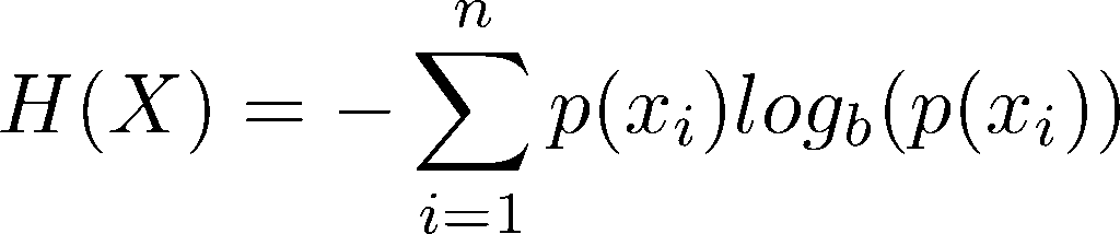
where x is a member of X and p(x) is a function to derive the probability of the value of x given the members present in X. b is the base of the logarithm, the appropriate value for which can vary depending on the use case. For our purposes of considering binary data, 2 is the best choice, as it maps to a bit being the smallest discrete unit we have of encoding information, the bit. n is the length of X. (We understand this terse, text-only explanation might not make the most sense to all readers; for a more visual explanation and to see how this equation is derived, check out this awesome StatQuest video).

We can go a step further once we know the entropy of the data string, and we can calculate the theoretical minimum bits we need to express the information contained in the original data by multiplying the entropy value by the length of the data string. Doing so tells us the theoretical number of bits a perfect entropy codec would require to express a given message, and thus a way to quantify the possible compressibility of the original string via an entropy codec by comparing the ratio of the original length in bits to the theoretical compressed length in bits.

Let’s see some examples of these calculations in practice! We’ll start with a simple 8-character string: AAAAAAAA:

• Length: 8
• Unique symbols: A
• Probability of A: p(A) = 8/8 = 1
• Entropy of string: H = -[ 1 * log₂(1) ] = -[ 1 * 0 ] = 0 bits/symbol
• Theoretical minimum length: 0 * 8 = 0 bits

This string is perfectly compressible, at least theoretically. Practically, a length of 0 seems a bit paradoxical, because how can we know what character to use and how many times to repeat it? Real entropy codecs cannot reach this theoretical minimum, but, especially with longer and more complex messages, modern algorithms are getting perilously close. Let’s try something a bit more complicated: ABBBABBB:

• Length: 8
• Unique symbols: A, B
• Probability of A: p(A) = 2/8 = 0.25
• Probability of B: p(B) = 6/8 = 0.75
• Entropy of string: H = -[ (0.25 * log₂(0.25)) + (0.75 * log₂(0.75)) ] = 0.811 bits/symbol
• Theoretical minimum length: 0.811 * 8 = 6.488 bits

If we assume ASCII encoding of our string ABBBABBB we know its length uncompressed is 8 bits per character, or 64 bits, almost ten times the theoretical minimum length. This tells us that entropy coding the ASCII encoding could theoretically get us a compression ratio of 10.

Let’s look at one more example, the array [ 0, 1, 2, 3, 4, 5, 6, 7 ]:

• Length: 8
• Unique symbols: 0, 1, 2, 3, 4, 5, 6, 7
• Probability of any symbol: p(x) = 1/8 = 0.125
• Entropy of string: H = -[ 8 * (0.125 * log₂(0.125)) ] = 3 bits/symbol
• Theoretical minimum length: 3 * 8 = 24 bits 

This is an interesting example. If we assume a naive data type like an 8-bit integer storing these values, then it looks like we do have some room for compression using entropy coding. Except, if we look more closely at the data, we see the minimum number of bits we need to express the range of integer values we have is three. That’s the same number of bits per symbol that entropy coding would have used! This array is actually not compressible using entropy coding, because there’s no redundancy in the data values for the coder to exploit!

Any compression here would actually be via bit-packing (packing our 8-bit values into 3-bits), not entropy coding. This is because bit-packing exploits the inefficiency of the data’s 8-bit container, while entropy coding exploits the statistical redundancy of the data’s values.

Does this mean we can’t compress this array?

It turns out this array is extremely compressible! The problem is that entropy coding looks at the data at “order-0” alone: each symbol is considered independently of all others. Said differently, if we can use other methods to find higher-order patterns within the data, then we can transform the data to remove those patterns to decrease the entropy of the array prior to entropy coding. If we reduce the data entropy without reducing the length, making the information less dense, then we’ll have entropy headroom our entropy codec can exploit to compress the data.

So how do we do this pattern matching and transformation? That brings us to the class of codecs called “predictors”.

Predictive codecs

A predictive codec, or “predictor” in common parlance, uses what it knows about the data it has seen so far to guess, or predict, other values in the dataset. Predictors output a “residual”, or the difference between the predicted value and the actual value.

A rather silly and simplistic example of this concept is to predict that the next value will simply be the same as the current value, and then store the difference. More formally:

predicted_value = previous_value
residual = current_value - predicted_value
residual = current_value - previous_value

Let’s see what this would look like applied to our previous example of the incompressible array:

• Given the array [ 0, 1, 2, 3, 4, 5, 6, 7 ] we start with the value 0
• Predicted next value is 0, residual is 1 - 0 = 1
• Predicted next value is 1, residual is 2 - 1 = 1
• Predicted next value is 2, residual is 3 - 2 = 1
• Predicted next value is 3, residual is 4 - 3 = 1
• …

The result of this silly predictor example is the array [ 0, 1, 1, 1, 1, 1, 1, 1 ]. But wait a minute, now we have a ton of redundancy. If we calculate the entropy of this new array we get 0.206 bits/symbol, giving us a theoretical minimum length of 1.651 bits. Compared to our prior 24-bit minimum length, this gives us a possible compression ratio of a little more than 14x!

If we want to get our original data back, we can easily reverse this transformation because it was lossless. We merely need to take the stored residuals and run a cumulative sum along the length of the array. In other words, current_value = previous_value + residual.

Turns out this “silly and simplistic” example is indeed simple, but isn’t so silly. What we just saw here is, basically, the operation of the numcodecs (Zarr) Delta codec and the transformation done by the TIFF predictor value 2. This “delta” transformation is frequently applied when compressing image data or non-image geospatial array data because it exploits the common higher-order pattern of spatial autocorrelation: values with close spatial proximity are more likely to be related than those far away from one another. Thus, using a neighboring value as a guess for the current value more often than not gets us pretty close, and does so in a way that can significantly reduce data variability, increasing redundancy and therefore compressibility.

Note that a delta predictor can be applied to an array in different ways. TIFF predictor 2, for example, specifically calculates the horizontal difference along rows by resetting the prediction at the start of each row. numcodecs Delta codec flattens an entire array into a single dimension, then calculates the difference along all values. One could imagine other potential ways to apply this difference, perhaps by calculating the vertical difference along columns, or by flattening an array using a space-filling curve like the Hilbert curve to maximally preserve locality in one dimension.

More complex predictor algorithms are also possible. Consider something like a moving window to allow more values to contribute to the prediction, or parameterized predictors that can be adjusted to more optimally map to the values in a specific dataset. ML models can also potentially be of value here by providing a means to facilitate highly adaptable automatic tuning of complex predictor models. The Burrows-Wheeler Transform (BWT) is a common predictor for compressing text data by reordering and grouping characters in a reversible way, and it or similar algorithms may also be applicable to geospatial array data.

In all of these examples the same principle applies: the extraction of higher-order patterns from a dataset in a reversible way can provide extreme reductions in entropy. Such processing is just as important to the compression process as entropy codecs.

Structural codecs

In addition to predictors, structural codecs are another important compression codec type. And we already saw one of these structural codecs make a cameo appearance in the discussion around entropy codecs: bit-packing!

Unlike predictors, bit-packing is itself something of a form of compression. Bit-packing allows us to push multiple values together by removing wasted space from byte-aligned in-memory data types. We previously saw the example of array [ 0, 1, 2, 3, 4, 5, 6, 7 ]. Storing these array values in memory requires maintaining byte alignment, so using an 8-bit integer type we end up with binary values like 0000 0000, 0000 0001, 0000 0010, …, 0000 0111. We see the leading 5 bits are always 0: they are unused except to provide padding to maintain a byte alignment. We can remove those unused bits when storing the data, because we don’t have the same per-value byte-alignment constraint on disk as we do when the values are loaded into memory for use.

numcodecs provides the PackBits codec to use bit-packing to condense boolean values together in this manner. GDAL supports a more flexible implementation of this concept for certain formats, such as GeoTIFF, using the NBITS option to get sub-byte data packing.

GDAL’s NBITS option is interesting because it can be used in a lossy manner: we could, for example, specify NBITS=2 when storing our example array and we’d reduce the length of the stored array by one third. That said, the loss of integer range would modify our data in a lossy manner as the array would become [ 0, 1, 2, 3, 0, 1, 2, 3 ].

NBITS actually hints at a key structural consideration when representing and compressing array data: what data type should be used in memory and on disk? Sometimes, as we see with NBITS and bit-packing, the answer is not the same for both. Generally speaking, integer types are well suited to most data, as they are easier to reason about than floating point types and do not suffer from precision/rounding errors or false precision. Even where data are decimal values, it can be advantageous to coerce them into a range that can be losslessly represented using an integer type to get processing efficiency and effectively fixed-precision representation. We’ll talk a bit more about how to do this coercion in the section on mapping codecs.

When it is necessary to store floating point values, however, it’s important to understand how floating point values work to then understand how we might be able to compress them more effectively. Let’s consider, for example, an array of the following four 32-bit floating point values, here represented in their binary forms:

• 01000001 01001000 00010001 00100010
• 01000001 01001000 11111111 11101110
• 01000001 01011100 00110011 01000100
• 01000001 01011100 10101010 10111011

In decimal form, the first of these is 12.5041828155517578125, but that’s a bit unwieldy. Let’s pretend for a moment that we’re only going to display six significant digits for these numbers. If we do so, our array becomes [ 12.5042, 12.5625, 13.7625, 13.7917 ]. If we want to compress this array using an entropy codec alone, we see we have no redundancy–each of the values are unique–so we’re already at the most compact form of these values. We could look at using a higher-order predictor like delta, which would give us [ 12.5042, 0.0583, 1.2000, 0.0294 ], but still we don’t see any obvious redundancy in this representation. What can we do?

The binary floats above are using the common IEEE 754 floating point representation. The 32-bit version of IEEE 754 stores a number using the following format: 1-bit sign, 8-bit exponent, 23-bit mantissa.

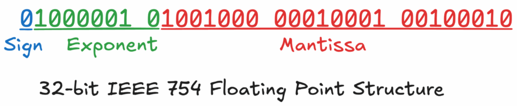
The important takeaway from the above is that, assuming spatial autocorrelation within our dataset, values close together typically have the same sign, the same or similar exponent values, and likely the same major mantissa components. In other words, the left-most bits of our values will generally have greater similarities, and the right-most bits will generally have greater variability. We can see this pattern across our four array values in their binary representations above.

We can make this left-to-right pattern exploitable by reordering the bytes within our floats, such that we group all the first byte values together, then the second bytes, third bytes, and finally the fourth byte values (like a pivot table). Our four groups in binary would then look like this:

• First bytes: 01000001 01000001 01000001 01000001
• Second bytes: 01001000 01001000 01011100 01011100
• Third bytes: 00010001 11111111 00110011 10101010
• Fourth bytes: 00100010 11101110 01000100 10111011

If we interpret these binary sequences into 8-bit integer values and concatenate them together into an array we get the following: [ 65, 65, 65, 65, 72, 72, 92, 92, 17, 255, 51, 170, 34, 238, 68, 187 ]. We can then run a delta predictor on this transformed representation to take advantage of the greater correlation in the reordered values: [ 65, 0, 0, 0, 7, 0, 20, 0, -75, 238, -204, 119, -136, 204, -170, 119 ]. As expected, we see greater variability and less repetition as we move right through the array. In other words, while the last few bytes remain noisy, the overall result is now dominated by zeros and small integers in the most significant parts of the data, and is meaningfully more compressible. On a realistic array with thousands of values, this effect becomes even more pronounced, potentially lowering entropy and increasing compressibility dramatically.

It turns out reordering bytes like in the above example is exactly what the numcodecs Shuffle codec does; its output can then be run through the Delta codec to replicate the full workflow here. And this combination of a shuffle operation with a delta is what TIFF predictor 3 does.

Structural codecs are always worthy of consideration in a compression pipeline in case they can better optimize data storage or emphasize structural patterns in a way that can help later operations compress more effectively. And not all structural codecs restructure the data based on its byte layout. For example, Run-Length Encoding (RLE) is a common content-based structural codec that compresses sequences of identical values, which can often be effective between delta or dictionary encoding and a final entropy codec.

Quantization/rounding codecs

Quantization codecs are lossy filters designed to reduce data size by permanently discarding insignificant precision. They achieve this by mapping a large set of input values to a smaller, more limited set.

The above floating point example still had quite a bit of variability in the least significant bits due to the way floats are stored internally. That is, IEEE 754 has 23 bits of fractional precision, which means we end up with many bits used to express really small pieces of our numbers to more precisely approximate the decimal values we are trying to store.

One way to remove much of the variability in those least significant bits is to quantize our values by setting some number of the least significant bits to all be zero. For our example, let’s say we want to zero the last 12 bits of our mantissas:

• 01000001 01001000 00010000 00000000: 12.50390625
• 01000001 01001000 11110000 00000000: 12.55859375
• 01000001 01011100 00110000 00000000: 13.76171875
• 01000001 01011100 10100000 00000000: 13.7890625

If we take these quantized values and do our shuffling and representation as 8-bit integers we get the following array: [ 65, 65, 65, 65, 72, 72, 92, 92, 16, 240, 48, 160, 0, 0, 0, 0 ]. And after a delta pass: [ 65, 0, 0, 0, 7, 0, 20, 0, -76, 224, -192, 112, -160, 0, 0, 0 ].

The result shows even more redundancy. Most significantly, because we zeroed out the entire last byte of precision, the final four values in our delta-encoded stream are now zero. We’ve also constrained the set of possible third-byte values from 256 to only 16. Both of these changes result in a dramatic increase in compressibility at the expense of precision. But note again: this is a lossy operation and we cannot reverse it.

Quantization can also be effective with integer data. Consider the example array [ 21, 46, 95, 147, 173 ]. Running delta on this gives us [ 21, 25, 49, 52, 26 ], which isn’t much help. If instead we were to round the values first: [ 20, 50, 100, 150, 170 ] → [ 20, 30, 50, 50, 20 ]. Now we see a meaningful improvement.

This idea of finding ways to throw away less significant information–noise–is a useful, if lossy, means of pre-processing to make later compression codec stages more effective. And we can do this using many different techniques. Traditional JPEG compression, for example, uses a frequency transform to identify and throw away higher frequency and thus lower value information within an image. Zarr’s numcodecs provides two codecs for quantization, Quantize and Bitround. Decimal rounding and variants, as we saw above, are also potentially effective mechanisms for quantization where they make sense. The lossy application of GDAL’s NBITS or numcodecs’ AsType could also be considered forms of quantization.

Mapping codecs

The last category of codecs we’re going to cover are mapping codecs. A mapping codec applies some sort of data transformation from a longer, more semantically-meaningful representation to a shorter, encoded form. Unlike entropy codecs, which map symbols to efficient bit codes, mapping codecs transform the data itself, typically by applying a static rule or lookup table to each value in isolation. Their primary goal is to simplify the “alphabet” of the data, making the subsequent job for predictors or entropy codecs much more effective.

A vast amount of array data uses mapping of some kind to encode the represented values. For example, images map some perceived reflectance as detected by a sensor to a numeric value. Or consider something like a land use raster: categories of use with semantic meaning are mapped to integer values for efficient array representation. Mappings are implicitly part of most raster array creation (and display, via a color map or color space).

We can be more explicit though with our use of mapping. For example, in the land use case, we could use something like numcodecs’ Categorize codec to make the mapping transformation part of our compression pipeline. We could potentially even leverage quantization here to coalesce related categories together in a lossy manner, increasing the redundancy and compressibility within the resulting dataset. For example, we could merge similar land use classes, e.g., by merging the more specific “deciduous forest” and “coniferous forest” classes to simply “forest”.

A related concept to simple category mapping is that of bitmaps. Bitmaps allow combining multiple classifications into a single integer value by mapping each bit in the integer to a specific category. For example, we could have a land use “forest” mapped to our least significant bit, and a protected status mapped to the next bit allowing us to indicate unprotected forest as 01, protected forest as 11, unprotected not forest as 00, and protected not forest as 10. Landsat QA bands use this bitmask technique to encode different QA flags into simple integer values. Zarr/numcodecs does not have a codec for bitmaps, but it seems like something here could be a valuable addition.

Another form of mapping is a mathematical/algorithmic approach. As we alluded to in the bitpacking discussion, we could use something like the numcodecs FixedScaleOffset codec to encode fixed point decimal values as integers. This codec takes two parameters, a scale and an offset, and calculates an encoded value via the equation encoded = (original - offset) * scale. For example, given the array [ 0.1, -0.5, 0.6, 1.7 ], we could use a scale of 10 and an offset of -1 to coerce our values into a range suitable for storing in an unsigned 8-bit integer. The result would be the scaled and offset array [ 11, 5, 16, 27 ], which now as integer values could be passed along to delta or other effective integer codec prior to the final entropy codec compression. The reverse of this lossless transformation is given by rewriting the previous equation: original = (encoded / scale) + offset.

GDAL also supports applying scale and offset when writing data to files that support embedding such metadata, like GeoTIFF. However, unlike Zarr, GDAL will not automatically reverse the transformation when reading data. In some ways this is good because this leaves the data in a more-efficient integer representation, but it can be misleading, particularly to users that are not familiar with this concept.

In addition to allowing fixed point values to be expressed as integers, scale and offset can also be used to map integer values into a smaller range. This technique is frequently leveraged to allow using a smaller data type. A common example of this could be the time dimension in CF conventions, which is often expressed as seconds since or days since the start time of the dataset’s observations.

How to benchmark compression

We previously delineated five key compression metrics: compression speed, decompression speed, memory footprint, compression ratio, compression lossiness, and compatibility. To fully benchmark a compression scheme we need to find some way to quantify each of these metrics.

The easiest of these to measure concretely are compression ratio and lossiness. Unlike speed or memory, the compression ratio and lossiness of a specific pipeline on some test array should be relatively constant across different operating systems, programming languages, and hardware platforms. Speed and memory, conversely, could vary significantly and in potentially profound and non-obvious ways (e.g., different library implementations, specialized CPU instruction sets, varying language overhead, etc.).

Compatibility is also not directly measurable by benchmarking tools. Certainly, having to use non-standard tooling is a good indication that a given codec is not going to be compatible with downstream applications, unless, of course, the codec is lossy and does not need to be reversed in any way. That said, even when using a standard tool to create a dataset, some options or codecs can make results incompatible with other tools or older tool versions (e.g., GDAL sparse GeoTIFFs, using zstd in TIFF files, etc.). As a result, understanding compatibility likely requires isolating a specific codec and format, such as “zstd support for TIFF”, then digging into various libraries, release versions, distro packaging, and high-level tooling to see how likely it is that a given set of users will be running compatible implementations (for the curious, zstd support was added to libtiff v4.0.10 in November 2018 with a unofficial compressor ID).

When running compression performance testing, be aware that comparing results across different array formats or different tooling can be potentially misleading, even when measured on the same machine. Treat such testing as a benchmark of the differences between different format software stacks by keeping the compression configuration constant. Doing so can be particularly difficult because different formats or tools may not support the exact same compression operations or parameters, in which case it is impossible to separate compression performance from the rest of the software stack.

Also, it’s helpful to note that underlying libraries used may not be the same depending on how each tool chain was compiled. Consider one such example: libtiff can be built to use libdeflate for faster DEFLATE performance, but Zarr’s equivalent GZip codec wraps the Python standard library gzip module, which is built against the less-optimized libzlib.

In this way, a set of truly ecosystem-wide benchmark results would be extremely complex to capture, if not impossible. This doesn’t mean that benchmarking is not important and would not be helpful. The libtiff v4.0.10 release notes mentioned above include a quite useful table comparing the different supported entropy codecs. But these results are still more incomplete than data producers really need: they are test dataset specific, and do not address any of the rest of the compression pipeline.

Wouldn’t it be great if data producers had tooling to help them better understand their datasets, and how best to compress them?

Zarrzipan

To this end, we’ve prototyped an experimental compression pipeline benchmarking tool called Zarrzipan. Zarrzipan is based on Zarr, borrowing the latter’s compression pipeline configuration format. It exposes both a CLI and a Python API to allow users to declaratively define compression pipelines and the arrays to run them against. All Zarr and numcodecs codecs are supported out of the box, and users can use Zarr’s codec extensibility to define their own custom codecs. All together, Zarrzipan allows users to experiment quickly and to quantitatively compare different pipelines across their own arrays.

The current implementation measures several different metrics, including compression and decompression times, memory usage, compression ratio, and lossiness. It allows users to average results over multiple iterations, if desired, and it also allows chunking input arrays to see how different chunking schemes affect the compression ratio. We’ve included a small set of example benchmarks of some Sentinel 2 compression pipelines in the repo README linked to above.

We believe Zarrzipan, or something like it, can serve as an effective tool for both learning about and experimenting with various compression techniques, as well as for evaluating optimal compression pipelines for various datasets. While the performance metrics might be specific to data stored in Zarr format, the principles should carry over to other formats.

Thinking beyond the default

Compression is a deeper and more multifaceted subject than is typically discussed. We’ve seen compression is much more than just entropy codecs, despite those seemingly getting all the attention. Pre-entropy-coding processing steps can be just as important to the overall compressibility of a dataset.

It’s particularly necessary for data providers to understand conceptually how all these pieces work together to ensure the data they are distributing is done so most efficiently and effectively. To support that need, we believe the community needs better resources to learn about and work with compression–Zarrzipan and this post are our initial contribution towards this goal.

Actually generating different compression pipeline possibilities and testing them with real, representative data, even with a tool like zarrzipan, can be a lot of hard work. Blosc has the btune tool to algorithmically explore and optimize along all possible compression dimensions, though this tool seems to be specific to blosc. Perhaps we need similar tooling for other formats.

Part of the difficulty, as has been mentioned, is the fragmentation of the ecosystem across all the various data formats, their libraries, and the underlying implementations. It seems like there’d be huge advantages to unifying the ecosystem onto one collection of codecs with verified optimal implementations, and using those codecs to read and write data across all formats. This is easier said than done, especially for legacy formats, but is part of the argument for a migration to Zarr, as its codec model seems the closest architecturally to this vision (even if implementations are still being optimized, and, at least from the outside, what is to happen with the numcodecs fracture appears uncertain at the moment).

This said, one of the most performant compression codecs supported by Zarr is blosc, and blosc2 appears to have been designed to be exactly this unified ecosystem. Blosc includes shuffle support, and also does chunking! Except it does so via a compiled library designed from the ground up for extreme performance via many optimization techniques. The overlaps between Zarr and blosc2 are somewhat hard to reconcile; perhaps this is a place to evaluate if blosc2 could be extended to support and offload all codec operations from Zarr. It seems like blosc2 is going this direction by supporting user-defined codecs; perhaps the pieces to support this idea are already in place, they just need to be leveraged by Zarr.

Amongst all of this compression complexity is one relatively simple point: array file formats are, in a sense, constraints on how data is compressed. The specific file format does not define the array data bytes on disk, that is a function of two things:

1. How the array is chunked
2. The compression pipeline

What compression operations can be performed on the data–what codecs are supported–is limited by the format, as is how the data can be chunked. As we showed in our previous post Is Zarr the new COG?, with equivalent chunking and compression the data bytes will be the same across formats. Thus, the major differences between array formats end up being:

• How metadata is stored, which drives the consequent flexibility/extensibility of the format
• The libraries that can read said metadata, what codec implementations they support, and the defaults they use

Note, however, that constraints are valuable, even perhaps more so than flexibility or extensibility. Constraints are a means of ensuring compatibility. In the wise words of Matt Hanson, “flexibility is the enemy of interoperability.” There’s a reason GeoTIFF using DEFLATE has been a go-to for so long, even if better compression is possible. But, in our cloud-native world with our ever-growing data volumes and network-dependent processing workloads, effective and efficient compression is perhaps more important than ever. Just accepting the defaults is no longer good enough, especially for major data producers. The community needs to ensure we are supporting users with sufficient documentation and tooling to have a good working understanding of compression and to make informed decisions about how best to compress their data. 

To discuss this idea further, reach out to our team directly on our contact page.